This project utilizes SQL and Python to conduct an analysis of a large database maintained by the Consumer Product Safety Commission (CPSC).
The following is an excerpt from the CPSC website about the NEISS project:
For more than 45 years, the CPSC has operated a statistically valid injury surveillance and follow-back system known as the National Electronic Injury Surveillance System (NEISS). The primary purpose of NEISS is to collect data on consumer product-related injuries occurring in the United States. CPSC uses these data to produce nationwide estimates of product-related injuries.

NEISS is based on a nationally representative probability sample of hospitals in the U.S. and its territories. Each participating NEISS hospital reports patient information for every emergency department visit associated with a consumer product or a poisoning to a child younger than five years of age. The total number of product-related hospital emergency department visits nationwide can be estimated from the sample of cases reported in the NEISS.

NEISS has become an important public health research tool, not just for CPSC, but also for researchers and consumers throughout the United States and around the world.
The raw data is available at: https://www.cpsc.gov/cgibin/NEISSQuery/.
Data Engineering
The NEISS query on the NEISS website outputs data as individual Excel files. The dimension tables are separated out of one Excel spreadsheet, and the fact tables are concatenated here with the code below. Each fact table file represents one year of data. They are ~40mb each and contain ~300,000 rows. The total size of all of the 20 Excel fact table files together is ~800mb. The maximum size for an excel sheet is just over 1,000,000 rows, so the data cannot be analyzed there. A tried and true method to analyze databases of this size is to use structured query language (SQL). This notebook uses SQL to input and output information from the database. It is used in tandem with Pandas to do aggregations and calculations. MatPlotLib and Seaborn are used for visualization.
Import the libraries
import os, time
import pandas as pd
import sqlite3
import numpy as np
import matplotlib.pyplot as plt
import seaborn as sns
Activate SQLite3
SQLite3 allows us to create a local .db file for quicker read and write times.
neiss_conn = sqlite3.connect('neiss.db')
Process raw excel files into a database
%%time
fact_directory = 'NEISS_All_Data/Fact Tables/'

dfs = []

# This code iterates through the list of documents in the directory
# and loads them into a list of dataframes. It was not working for
# me at the time because the files were being loaded to the cloud
# in the middle of processing.
'''
for filename in os.listdir(fact_directory):
    filename_l = filename.lower()
    if filename_l.endswith('xlsx') and filename_l.startswith('neiss'):
        filepath = os.path.join(fact_directory, filename)
        df = pd.read_excel(filepath)
        dfs.append(df)
data_load_finish = time.time() - start_time
print(data_load_finish)

# Concatenate the list of dataframes into one large dataframe
neiss_all = pd.concat(dfs, ignore_index=True)
'''

# Loads the files individually and processes them into the database
df = pd.read_excel('NEISS_All_Data/Fact Tables/NEISS_2003.XLSX')
df.to_sql('neiss_all', neiss_conn, if_exists = 'append', index=True)
CPU times: user 1min 39s, sys: 5.12 s, total: 1min 44s
Wall time: 1min 47s
347375
Check the fact table data
%%time

neiss_all = pd.read_sql(
'''

SELECT * FROM neiss_all

'''
,neiss_conn)
neiss_all
CPU times: user 1min 3s, sys: 30 s, total: 1min 33s
Wall time: 1min 33s
| index | CPSC_Case_Number | Treatment_Date | Age | Sex | Race | Other_Race | Hispanic | Body_Part | Diagnosis | ... | Product_2 | Product_3 | Narrative | Stratum | PSU | Weight | Other_Diagnosis | Other_Diagnosis_2 | year | Product_All | |
|---|---|---|---|---|---|---|---|---|---|---|---|---|---|---|---|---|---|---|---|---|---|
| 0 | 0 | 90101432 | 2009-01-01 00:00:00 | 5 | 1 | 3 | HISPANIC | NaN | 89 | 64 | ... | 0 | 0 | 5 YOM ROLLING ON FLOOR DOING A SOMERSAULT AND ... | V | 61 | 15.3491 | None | None | 2009 | None |
| 1 | 1 | 90101434 | 2009-01-01 00:00:00 | 51 | 1 | 1 | None | NaN | 77 | 53 | ... | 0 | 0 | 51 YOM C/O PAIN AND IRRITATION TO RIGHT EYE, H... | V | 61 | 15.3491 | None | None | 2009 | None |
| 2 | 2 | 90101435 | 2009-01-01 00:00:00 | 2 | 2 | 1 | None | NaN | 76 | 59 | ... | 0 | 0 | 2 YOF WAS RUNNING THROUGH HOUSE AND FELL INTO ... | V | 61 | 15.3491 | None | None | 2009 | None |
| 3 | 3 | 90101436 | 2009-01-01 00:00:00 | 20 | 1 | 1 | None | NaN | 93 | 53 | ... | 0 | 0 | 20 YOM PUNCHED AND KICKED A WALL D/T DRINKING ... | V | 61 | 15.3491 | None | None | 2009 | None |
| 4 | 4 | 90101437 | 2009-01-01 00:00:00 | 20 | 1 | 1 | None | NaN | 34 | 57 | ... | 0 | 0 | 20 YOM FELL SNOW SKIING SUSTAINING A FRACTURED... | V | 61 | 15.3491 | None | None | 2009 | None |
| ... | ... | ... | ... | ... | ... | ... | ... | ... | ... | ... | ... | ... | ... | ... | ... | ... | ... | ... | ... | ... | ... |
| 7316556 | 347370 | 40605786 | 2003-05-31 00:00:00 | 2 | 2 | 2 | None | NaN | 76 | 53 | ... | 0 | 0 | PATIENT PULLED HAMMER DOWN AND HIT EYE; FACIAL... | C | 8 | 6.1043 | None | None | 2003 | None |
| 7316557 | 347371 | 40605787 | 2003-05-31 00:00:00 | 206 | 2 | 1 | None | NaN | 30 | 53 | ... | 4057 | 0 | BABYSITTER DROPPED PATIENT ONTO FLOOR, HIT LEF... | C | 8 | 6.1043 | None | None | 2003 | None |
| 7316558 | 347372 | 40605789 | 2003-05-31 00:00:00 | 2 | 2 | 2 | None | NaN | 76 | 59 | ... | 4057 | 0 | PATIENT FELL OFF COUCH HITTING HEAD ON WOODEN ... | C | 8 | 6.1043 | None | None | 2003 | None |
| 7316559 | 347373 | 40605791 | 2003-05-31 00:00:00 | 11 | 1 | 2 | None | NaN | 76 | 59 | ... | 1871 | 0 | PATIENT PLAYING BASKETBALL, FELL INTO METAL FE... | C | 8 | 6.1043 | None | None | 2003 | None |
| 7316560 | 347374 | 40605792 | 2003-05-31 00:00:00 | 10 | 2 | 3 | UNKNOWN | NaN | 92 | 53 | ... | 0 | 0 | PATIENT HAD PREVIOUSLY INJURED HAND WHILE PLAY... | C | 8 | 6.1043 | None | None | 2003 | None |
7316561 rows × 30 columns
neiss_all.info()
<class 'pandas.core.frame.DataFrame'>
RangeIndex: 7316561 entries, 0 to 7316560
Data columns (total 30 columns):
 #   Column             Dtype
---  ------             -----
 0   index              int64
 1   CPSC_Case_Number   int64
 2   Treatment_Date     object
 3   Age                int64
 4   Sex                int64
 5   Race               int64
 6   Other_Race         object
 7   Hispanic           float64
 8   Body_Part          int64
 9   Diagnosis          int64
 10  Diagoth            object
 11  Body_Part_2        float64
 12  Diagnosis_2        float64
 13  Diag2oth           object
 14  Disposition        int64
 15  Location           int64
 16  Fire_Involvement   int64
 17  Alcohol            float64
 18  Drug               float64
 19  Product_1          int64
 20  Product_2          int64
 21  Product_3          int64
 22  Narrative          object
 23  Stratum            object
 24  PSU                int64
 25  Weight             float64
 26  Other_Diagnosis    object
 27  Other_Diagnosis_2  object
 28  year               int64
 29  Product_All        object
dtypes: float64(6), int64(15), object(9)
memory usage: 1.6+ GB
This is the schema for the fact table. There are over 7 million rows and 27 columns.
%%time

# This query is to make sure that all of the files made it to the database

view = pd.read_sql(

'''

SELECT DISTINCT SUBSTRING(Treatment_Date, 1, 4) AS first_four_digits
FROM neiss_all
ORDER BY first_four_digits Desc


'''
,neiss_conn)
view
CPU times: user 1.84 s, sys: 1.1 s, total: 2.95 s
Wall time: 3.55 s
| first_four_digits | |
|---|---|
| 0 | 2022 |
| 1 | 2021 |
| 2 | 2020 |
| 3 | 2019 |
| 4 | 2018 |
| 5 | 2017 |
| 6 | 2016 |
| 7 | 2015 |
| 8 | 2014 |
| 9 | 2013 |
| 10 | 2012 |
| 11 | 2011 |
| 12 | 2010 |
| 13 | 2009 |
| 14 | 2008 |
| 15 | 2007 |
| 16 | 2006 |
| 17 | 2005 |
| 18 | 2004 |
| 19 | 2003 |
Check for duplicates
%%time

neiss_all = pd.read_sql(
'''

SELECT DISTINCT *
from neiss_all

'''
,neiss_conn)
neiss_all
CPU times: user 1min 27s, sys: 50.2 s, total: 2min 17s
Wall time: 2min 23s
| index | CPSC_Case_Number | Treatment_Date | Age | Sex | Race | Other_Race | Hispanic | Body_Part | Diagnosis | ... | Drug | Product_1 | Product_2 | Product_3 | Narrative | Stratum | PSU | Weight | Other_Diagnosis | Other_Diagnosis_2 | |
|---|---|---|---|---|---|---|---|---|---|---|---|---|---|---|---|---|---|---|---|---|---|
| 0 | 0 | 90101432 | 2009-01-01 00:00:00 | 5 | 1 | 3 | HISPANIC | NaN | 89 | 64 | ... | NaN | 1807 | 0 | 0 | 5 YOM ROLLING ON FLOOR DOING A SOMERSAULT AND ... | V | 61 | 15.3491 | None | None |
| 1 | 1 | 90101434 | 2009-01-01 00:00:00 | 51 | 1 | 1 | None | NaN | 77 | 53 | ... | NaN | 899 | 0 | 0 | 51 YOM C/O PAIN AND IRRITATION TO RIGHT EYE, H... | V | 61 | 15.3491 | None | None |
| 2 | 2 | 90101435 | 2009-01-01 00:00:00 | 2 | 2 | 1 | None | NaN | 76 | 59 | ... | NaN | 4057 | 0 | 0 | 2 YOF WAS RUNNING THROUGH HOUSE AND FELL INTO ... | V | 61 | 15.3491 | None | None |
| 3 | 3 | 90101436 | 2009-01-01 00:00:00 | 20 | 1 | 1 | None | NaN | 93 | 53 | ... | NaN | 1884 | 0 | 0 | 20 YOM PUNCHED AND KICKED A WALL D/T DRINKING ... | V | 61 | 15.3491 | None | None |
| 4 | 4 | 90101437 | 2009-01-01 00:00:00 | 20 | 1 | 1 | None | NaN | 34 | 57 | ... | NaN | 3283 | 0 | 0 | 20 YOM FELL SNOW SKIING SUSTAINING A FRACTURED... | V | 61 | 15.3491 | None | None |
| ... | ... | ... | ... | ... | ... | ... | ... | ... | ... | ... | ... | ... | ... | ... | ... | ... | ... | ... | ... | ... | ... |
| 7316556 | 347370 | 40605786 | 2003-05-31 00:00:00 | 2 | 2 | 2 | None | NaN | 76 | 53 | ... | NaN | 827 | 0 | 0 | PATIENT PULLED HAMMER DOWN AND HIT EYE; FACIAL... | C | 8 | 6.1043 | None | None |
| 7316557 | 347371 | 40605787 | 2003-05-31 00:00:00 | 206 | 2 | 1 | None | NaN | 30 | 53 | ... | NaN | 1807 | 4057 | 0 | BABYSITTER DROPPED PATIENT ONTO FLOOR, HIT LEF... | C | 8 | 6.1043 | None | None |
| 7316558 | 347372 | 40605789 | 2003-05-31 00:00:00 | 2 | 2 | 2 | None | NaN | 76 | 59 | ... | NaN | 679 | 4057 | 0 | PATIENT FELL OFF COUCH HITTING HEAD ON WOODEN ... | C | 8 | 6.1043 | None | None |
| 7316559 | 347373 | 40605791 | 2003-05-31 00:00:00 | 11 | 1 | 2 | None | NaN | 76 | 59 | ... | NaN | 1205 | 1871 | 0 | PATIENT PLAYING BASKETBALL, FELL INTO METAL FE... | C | 8 | 6.1043 | None | None |
| 7316560 | 347374 | 40605792 | 2003-05-31 00:00:00 | 10 | 2 | 3 | UNKNOWN | NaN | 92 | 53 | ... | NaN | 5041 | 0 | 0 | PATIENT HAD PREVIOUSLY INJURED HAND WHILE PLAY... | C | 8 | 6.1043 | None | None |
7316561 rows × 28 columns
In this case there are no duplicates, but if we wanted to create a table with no duplicates, the SQL code would be:
create a temporary table:
CREATE TABLE neiss_WO_duplicates AS
SELECT DISTINCT
FROM neiss_all
then drop the table with duplicates:
DROP TABLE neiss_all
rename the table:
ALTER TABLE neiss_WO_duplicates RENAME TO neiss_all
This would need to be done via neiss_conn.execute()
neiss_conn.commit() is used to commit the changes to the database
# Writes the dataframe to the sql file

neiss_all.to_sql('neiss_all', neiss_conn, index=True)
Extract the Year
The year is extracted from the Treatment_Date column for easy analysis
Add the year column to the table
neiss_conn.execute(
'''

ALTER TABLE neiss_all
ADD COLUMN year INT

'''
)
<sqlite3.Cursor at 0x7fe963223420>
Calculate the values from the date column
neiss_conn.execute(
'''

UPDATE neiss_all
SET year = strftime('%Y',Treatment_Date)

'''
)
<sqlite3.Cursor at 0x7fe92745ef80>
Because we are using SQLite3, we are required to use strftime() to handle date/time information. YEAR([column]) would work in most other SQL implementations.
'%Y' is capitalized to represent that we need a four-digit year.
view = pd.read_sql(
'''

SELECT DISTINCT year
FROM neiss_all


'''
,neiss_conn)

view.values
array([[2009],
       [2005],
       [2013],
       [2012],
       [2022],
       [2021],
       [2020],
       [2019],
       [2018],
       [2017],
       [2016],
       [2015],
       [2014],
       [2011],
       [2010],
       [2008],
       [2007],
       [2006],
       [2004],
       [2003]])
There are no null or 0 values
# Commit the changes to the database
neiss_conn.commit()
View the column information as SQL code
# Set the pandas display.max_colwidth attribute to None
# so the entire contents of the cell can be seen
pd.set_option('display.max_colwidth', None)

# The is SQL query returns the columns with their types in the style
# of a SQL code
view = pd.read_sql(
'''

SELECT sql FROM sqlite_master WHERE type = 'table' AND name = 'neiss_all';


'''
,neiss_conn)
view
| sql | |
|---|---|
| 0 | CREATE TABLE "all_neiss" (\n"index" INTEGER,\n "CPSC_Case_Number" INTEGER,\n "Treatment_Date" TIMESTAMP,\n "Age" INTEGER,\n "Sex" INTEGER,\n "Race" INTEGER,\n "Other_Race" TEXT,\n "Hispanic" REAL,\n "Body_Part" INTEGER,\n "Diagnosis" INTEGER,\n "Diagoth" TEXT,\n "Body_Part_2" REAL,\n "Diagnosis_2" REAL,\n "Diag2oth" REAL,\n "Disposition" INTEGER,\n "Location" INTEGER,\n "Fire_Involvement" INTEGER,\n "Alcohol" REAL,\n "Drug" REAL,\n "Product_1" INTEGER,\n "Product_2" INTEGER,\n "Product_3" INTEGER,\n "Narrative" TEXT,\n "Stratum" TEXT,\n "PSU" INTEGER,\n "Weight" REAL,\n "Other_Diagnosis" TEXT,\n "Other_Diagnosis_2" REAL\n, year INT) |
# Reset the pandas column width setting back to default.
pd.reset_option('display.max_colwidth')
Combine Columns
In the fact table we have three columns: Product_1, Product_2, and Product_3. The second two columns provide additional input areas if more than one product was involved in an injury. We will combine these columns so that we can get the complete view of the products variable. In this case, a new table will be created, but similar operations will be conducted later in the notebook, and they are usually saved in the form of a View.
Note that aggregations containing more than product category will no longer perfectly represent the number of cases, but will instead represent the number of times that the specific products were listed. In the cases the the product is filtered down to one category, the aggregation will represent the number of cases.
First we will see how much the size of the data set will increase if we add the additional columns
# View the count of the three columns, when they are not equal to 0

view = pd.read_sql(
'''

SELECT COUNT(CASE WHEN Product_1 <> 0 THEN 1 ELSE NULL END)
     + COUNT(CASE WHEN Product_2 <> 0 THEN 1 ELSE NULL END)
     + COUNT(CASE WHEN Product_3 <> 0 THEN 1 ELSE NULL END) AS count
FROM neiss_all;


'''
, neiss_conn)
view
| count | |
|---|---|
| 0 | 8313005 |
The output table would only be about a million rows larger than our current table. This is manageable, so we will proceed.
Code notes:
- UNION ALL is used to concatenate tables. Without ALL, the UNION operation eliminates any duplicate rows.
- Table_name.* can be used to select all of the columns in the table, and also add additional columns.
- In each of the three tables joined in the subquery, 0's are filtered so that there are no unnecessary duplicates.
neiss_conn.execute(
'''

CREATE TABLE neiss_prod AS
SELECT *
FROM (
    SELECT neiss_all.*, product_1 AS Product_All
    FROM neiss_all
    WHERE Product_1 != 0
    UNION ALL
    SELECT neiss_all.*, product_2 AS Product_All
    FROM neiss_all
    WHERE Product_2 != 0
    UNION ALL
    SELECT neiss_all.*, product_3 AS Product_All
    FROM neiss_all
    WHERE Product_3 != 0

) AS Subquery


'''
)
view = pd.read_sql(
'''

SELECT *
FROM neiss_prod


'''
, neiss_conn)
view
| index | CPSC_Case_Number | Treatment_Date | Age | Sex | Race | Other_Race | Hispanic | Body_Part | Diagnosis | ... | Product_2 | Product_3 | Narrative | Stratum | PSU | Weight | Other_Diagnosis | Other_Diagnosis_2 | year | Product_All | |
|---|---|---|---|---|---|---|---|---|---|---|---|---|---|---|---|---|---|---|---|---|---|
| 0 | 0 | 90101432 | 2009-01-01 00:00:00 | 5 | 1 | 3 | HISPANIC | NaN | 89 | 64 | ... | 0 | 0 | 5 YOM ROLLING ON FLOOR DOING A SOMERSAULT AND ... | V | 61 | 15.3491 | None | None | 2009 | 1807 |
| 1 | 1 | 90101434 | 2009-01-01 00:00:00 | 51 | 1 | 1 | None | NaN | 77 | 53 | ... | 0 | 0 | 51 YOM C/O PAIN AND IRRITATION TO RIGHT EYE, H... | V | 61 | 15.3491 | None | None | 2009 | 899 |
| 2 | 2 | 90101435 | 2009-01-01 00:00:00 | 2 | 2 | 1 | None | NaN | 76 | 59 | ... | 0 | 0 | 2 YOF WAS RUNNING THROUGH HOUSE AND FELL INTO ... | V | 61 | 15.3491 | None | None | 2009 | 4057 |
| 3 | 3 | 90101436 | 2009-01-01 00:00:00 | 20 | 1 | 1 | None | NaN | 93 | 53 | ... | 0 | 0 | 20 YOM PUNCHED AND KICKED A WALL D/T DRINKING ... | V | 61 | 15.3491 | None | None | 2009 | 1884 |
| 4 | 4 | 90101437 | 2009-01-01 00:00:00 | 20 | 1 | 1 | None | NaN | 34 | 57 | ... | 0 | 0 | 20 YOM FELL SNOW SKIING SUSTAINING A FRACTURED... | V | 61 | 15.3491 | None | None | 2009 | 3283 |
| ... | ... | ... | ... | ... | ... | ... | ... | ... | ... | ... | ... | ... | ... | ... | ... | ... | ... | ... | ... | ... | ... |
| 8313000 | 358454 | 200306247 | 2019-08-16 00:00:00 | 3 | 1 | 2 | None | 2.0 | 31 | 48 | ... | 264 | 1135 | 3YOM WITH BURN, PUT HOT CUP OF WATER/TEA OUT O... | C | 10 | 4.8283 | None | None | 2019 | 1135 |
| 8313001 | 358460 | 200306262 | 2019-08-17 00:00:00 | 3 | 1 | 1 | None | 2.0 | 75 | 62 | ... | 1807 | 676 | 3YOM FELL 4-5 STAIRS DOWN CARPETED STAIRS ONTO... | C | 10 | 4.8283 | None | None | 2019 | 676 |
| 8313002 | 358577 | 200308374 | 2019-09-16 00:00:00 | 209 | 1 | 1 | None | 1.0 | 75 | 62 | ... | 1807 | 676 | 9MOM ROLLED OFF BED (2FT HIGH) ONTO CARPET FLO... | C | 10 | 4.8283 | None | None | 2019 | 676 |
| 8313003 | 358662 | 200314181 | 2019-12-31 00:00:00 | 67 | 2 | 4 | None | 2.0 | 75 | 62 | ... | 4076 | 1884 | 67YOF P/W BLEEDING TO BACK OF HEADF AFTER FALL... | V | 57 | 17.3778 | None | None | 2019 | 1884 |
| 8313004 | 358685 | 200314472 | 2019-07-30 00:00:00 | 4 | 1 | 1 | None | 1.0 | 85 | 68 | ... | 4076 | 1131 | 4YOM WAS FOUND BY HIS MOTHER SLEEPING IN HIS B... | S | 65 | 84.0408 | None | None | 2019 | 1131 |
8313005 rows × 30 columns
The number of rows matches our calculation from earlier. The operation is a success.
neiss_conn.commit()
Load the dimension tables
There are a total of 11 dimension tables. The largest is the product dimension table with about 1100 rows.
dim_directory = 'NEISS_All_Data/Dimension Tables/'
dataframes = {}

# Loads the dimension tables into a dictionary

for filename in os.listdir(dim_directory):
    if filename.endswith('.xlsx'):
        filepath = os.path.join(dim_directory, filename)
        dataframe_name = filename.split('.')[0]  # Use the filename as the dataframe name
        dataframes[dataframe_name] = pd.read_excel(filepath)
Upload the dimension tables into the database
for dataframe_name, dataframe in dataframes.items():
    dataframe.to_sql(dataframe_name, neiss_conn, if_exists='replace', index=False)
View all of the tables in the database
view = pd.read_sql(
'''

SELECT name FROM sqlite_master WHERE type='table'

'''
,neiss_conn)
view
| name | |
|---|---|
| 0 | neiss_all |
| 1 | AgeLTwoDim |
| 2 | DispositionDim |
| 3 | RaceDim |
| 4 | FireDim |
| 5 | LocationDim |
| 6 | GenderDim |
| 7 | HispanicDim |
| 8 | BdypartDim |
| 9 | DiagnosisDim |
| 10 | Alc_DrugDim |
| 11 | ProductDim |
| 12 | neiss_prod |
Analysis
What is the total number of injuries on record?
Starting off simple, we get the total count for the number of cases. The count is given the alias 'Total_Count'. This will match the row count.
view = pd.read_sql(
'''

SELECT count(CPSC_Case_Number) as Total_Count
FROM neiss_all

'''
,neiss_conn
)
view
| Total_Count | |
|---|---|
| 0 | 7316561 |
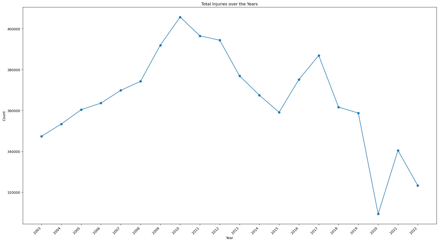
How is the total number of injuries changing over time?
This code is essentially the same as the first, but in this case a GROUP BY statement is added to aggregate the count according to the year.
view = pd.read_sql(
'''

SELECT year, count(CPSC_Case_Number) as count
FROM neiss_all
GROUP BY year

'''
,neiss_conn
)
view
| year | count | |
|---|---|---|
| 0 | 2003 | 347375 |
| 1 | 2004 | 353388 |
| 2 | 2005 | 360372 |
| 3 | 2006 | 363609 |
| 4 | 2007 | 369832 |
| 5 | 2008 | 374260 |
| 6 | 2009 | 391944 |
| 7 | 2010 | 405710 |
| 8 | 2011 | 396502 |
| 9 | 2012 | 394383 |
| 10 | 2013 | 376926 |
| 11 | 2014 | 367492 |
| 12 | 2015 | 359129 |
| 13 | 2016 | 375196 |
| 14 | 2017 | 386906 |
| 15 | 2018 | 361667 |
| 16 | 2019 | 358715 |
| 17 | 2020 | 309370 |
| 18 | 2021 | 340442 |
| 19 | 2022 | 323343 |
This code creates a line plot to view the results.
# Change from view to df to avoid confusion
df = view

# Create the plot
fig, ax = plt.subplots(figsize=(18, 10))
df.sort_values('year')
df.plot(kind='line', ax=ax, marker='o', x='year',y='count', legend=False)

# Set the axis labels
ax.set_xlabel('Year')
ax.set_ylabel('Count')
ax.set_title('Total Injuries over the Years')

# Set the tick marks to avoid decimal numbers, set the rotation, and align the text
ax.set_xticks(view['year'].unique())
ax.set_xticklabels(view['year'].unique(), rotation=45, ha='right')


plt.tight_layout()

plt.show()
print(view[(view['year']==2022)].values - view[(view['year']==2003)].values)
print(view[(view['year']==2022)].values - view[(view['year']==2010)].values)
[[    19 -24032]]
[[    12 -82367]]
Notes:
- The number of injuries has been on the decline since it's peak of 405,710 in 2010.
- Overall, there has been a decrease of 24,032 since 2003, and 82,367 since 2010.
- There was a significant drop 2020, the year the Covid Pandemic began.
Which products created the most injuries?
Top 20 of all time
%%time
Top_20 = pd.read_sql(
'''

SELECT PRODUCT, count(CPSC_Case_Number) count
FROM neiss_prod
LEFT JOIN ProductDim on Code = Product_All
GROUP BY Product_All
ORDER BY count Desc
LIMIT 20

'''
,neiss_conn
)
Top_20
CPU times: user 3.4 s, sys: 664 ms, total: 4.07 s
Wall time: 4.08 s
| PRODUCT | count | |
|---|---|---|
| 0 | FLOORS OR FLOORING MATERIALS | 769700 |
| 1 | STAIRS OR STEPS | 630429 |
| 2 | BEDS OR BEDFRAMES, OTHER OR NOT SPECIFIED | 365585 |
| 3 | BASKETBALL, ACTIVITY AND RELATED EQUIPMENT | 287608 |
| 4 | BICYCLES AND ACCESSORIES, (EXCL.MOUNTAIN OR AL... | 272479 |
| 5 | FOOTBALL (ACTIVITY, APPAREL OR EQUIPMENT) | 235824 |
| 6 | CEILINGS AND WALLS (INTERIOR PART OF COMPLETED... | 193580 |
| 7 | TABLES (EXCL. BABY CHANGING TABLES, BILLIARD ... | 193075 |
| 8 | CHAIRS, OTHER OR NOT SPECIFIED | 186006 |
| 9 | DOORS, OTHER OR NOT SPECIFIED | 175816 |
| 10 | KNIVES, NOT ELSEWHERE CLASSIFIED | 165347 |
| 11 | BATHTUBS OR SHOWERS | 149746 |
| 12 | SOCCER (ACTIVITY, APPAREL OR EQUIPMENT) | 126562 |
| 13 | EXERCISE (ACTIVITY OR APPAREL, W/O EQUIP) | 126131 |
| 14 | SOFAS, COUCHES, DAVENPORTS, DIVANS OR STUDIO C... | 111686 |
| 15 | FOOTWEAR | 93780 |
| 16 | CABINETS, RACKS, ROOM DIVIDERS AND SHELVES, NEC | 79890 |
| 17 | LADDERS, OTHER OR NOT SPECIFIED | 77042 |
| 18 | RUGS OR CARPETS, NOT SPECIFIED | 74474 |
| 19 | BASEBALL (ACTIVITY, APPAREL OR EQUIPMENT; EXCL... | 72918 |
Notes:
- Floors and stairs are at the top of the list at 770k and 630k respectively. Stairs has nearly twice the number as the next product down, which was beds at 366k.
- Sports are a common cause of injury, but all of the sports related injuries combined add up to roughly the number of floor-related injuries
- Bed-related injuries are very common considering they usually involve sedentary activities.
Top 20 over time
The code below creates and calls from a subquery in which row numbers are assigned to a partition designated by the year number, and ordered by the count of the case number in descending order. That means there will be a series from 1 to 1,122 (the number of products) for 2003, 1 to 1,122 for 2004 and so on. This labelling is stored in a temporary column called rn, which can be used to designate how many products to include for each year.
The subquery effectively acts as a table to be called from and manipulated.
view = pd.read_sql(
'''

SELECT year, prod.PRODUCT, count
FROM (
    SELECT year, Product_All, count(CPSC_Case_Number) as count,
           ROW_NUMBER() OVER (PARTITION BY year ORDER BY count(CPSC_Case_Number) DESC) as rn
    FROM neiss_prod
    GROUP BY year, Product_All
) subquery
LEFT JOIN ProductDim AS prod ON prod.Code = subquery.Product_All
WHERE rn <= 15
ORDER BY year, count DESC


'''
, neiss_conn)
view
| year | PRODUCT | count | |
|---|---|---|---|
| 0 | 2003 | STAIRS OR STEPS | 29254 |
| 1 | 2003 | FLOORS OR FLOORING MATERIALS | 27460 |
| 2 | 2003 | BASKETBALL, ACTIVITY AND RELATED EQUIPMENT | 16928 |
| 3 | 2003 | BICYCLES AND ACCESSORIES, (EXCL.MOUNTAIN OR AL... | 15101 |
| 4 | 2003 | BEDS OR BEDFRAMES, OTHER OR NOT SPECIFIED | 13101 |
| ... | ... | ... | ... |
| 295 | 2022 | KNIVES, NOT ELSEWHERE CLASSIFIED | 6697 |
| 296 | 2022 | EXERCISE (ACTIVITY OR APPAREL, W/O EQUIP) | 6676 |
| 297 | 2022 | SOCCER (ACTIVITY, APPAREL OR EQUIPMENT) | 6308 |
| 298 | 2022 | DOORS, OTHER OR NOT SPECIFIED | 6305 |
| 299 | 2022 | SOFAS, COUCHES, DAVENPORTS, DIVANS OR STUDIO C... | 5870 |
300 rows × 3 columns
This code is to create a line chart from the data given above. The data is pivoted so the .plot() method can read it as a dataframe. The total count for each product across all years is calculated, and then the index is applied so that the data is sorted like the first table table above.
# Convert the 'year' column to integers
view['year'] = view['year'].astype(int)

# Pivot the data to have products as columns and years as rows
pivot_data = view.pivot(index='year', columns='PRODUCT', values='count')

# Calculate the total count for each product across all years
product_totals = pivot_data.sum().sort_values(ascending=False)

# Sort the pivot_data columns based on the product_totals order
pivot_data = pivot_data[product_totals.index]

# Plot the line chart and add details
fig, ax = plt.subplots(figsize=(15, 10))
pivot_data.plot(kind='line', ax=ax, marker='o')

ax.set_xlabel('Year')
ax.set_ylabel('Count')
ax.set_title('Products Contributing to Injuries Over the Years (Top 15 Every Year)')

# Adjust the x-tick labels so they are angled and don't overlap
ax.set_xticks(view['year'].unique())
ax.set_xticklabels(view['year'].unique(), rotation=45, ha='right')

# Move the legend below the plot
ax.legend(title='Product', bbox_to_anchor=(0.5, -0.2), loc='upper center', ncol=3)

plt.tight_layout()

plt.show()
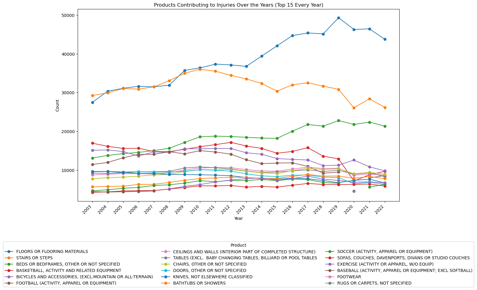
Notes:
- The number of injuries due to floors or flooring materials has increased dramatically over the past 20 years.
- Basketball-related injuries have steadily decreased since 2003 and sharply decreased in 2020.
- Bed-related injuries have steadily increased.
- Stair related injuries have been decreasing since 2010.
- Bicycle-related injuries have slowly been decreasing since 2003.
This is a table comparing 2003 to 2022 values. Products that weren't in the top 15 for either of those years have been dropped.
The code uses python to pivot the data and add two calculated columns. Then, a new dataframe is created with the appropriate column names so that the dataframe format is simplified and columns can be called by their respective names. Null values are then dropped and then the data is sorted according to 2022 values.
subselection = view[view['year'].isin([2003, 2022])]

# Group by product and pivot the table to have years as columns
pivot_table = subselection.pivot_table(index='PRODUCT', columns='year', values='count', aggfunc='sum')

# Calculate the difference between 2022 and 2003
pivot_table['difference'] = pivot_table[2022] - pivot_table[2003]

# Calculate the quotient for 2022 over 2003
pivot_table['quotient'] = pivot_table[2022] / pivot_table[2003] -1

# Create the new DataFrame with the desired columns
new_df = pd.DataFrame({'2003': pivot_table[2003],'2022': pivot_table[2022], 'difference': pivot_table['difference'], '%change': pivot_table['quotient']})

# Drop rows with null values and order by 2022
new_df = new_df.dropna().sort_values(by='2022',ascending=False)

# Display the new DataFrame
new_df
| 2003 | 2022 | difference | %change | |
|---|---|---|---|---|
| PRODUCT | ||||
| FLOORS OR FLOORING MATERIALS | 27460.0 | 43784.0 | 16324.0 | 0.594465 |
| STAIRS OR STEPS | 29254.0 | 26172.0 | -3082.0 | -0.105353 |
| BEDS OR BEDFRAMES, OTHER OR NOT SPECIFIED | 13101.0 | 21332.0 | 8231.0 | 0.628273 |
| BICYCLES AND ACCESSORIES, (EXCL.MOUNTAIN OR ALL-TERRAIN) | 15101.0 | 9807.0 | -5294.0 | -0.350573 |
| BASKETBALL, ACTIVITY AND RELATED EQUIPMENT | 16928.0 | 9670.0 | -7258.0 | -0.428757 |
| CHAIRS, OTHER OR NOT SPECIFIED | 7753.0 | 8906.0 | 1153.0 | 0.148717 |
| CEILINGS AND WALLS (INTERIOR PART OF COMPLETED STRUCTURE) | 8739.0 | 8656.0 | -83.0 | -0.009498 |
| FOOTBALL (ACTIVITY, APPAREL OR EQUIPMENT) | 11434.0 | 8565.0 | -2869.0 | -0.250918 |
| TABLES (EXCL. BABY CHANGING TABLES, BILLIARD OR POOL TABLES | 9190.0 | 8282.0 | -908.0 | -0.098803 |
| BATHTUBS OR SHOWERS | 5668.0 | 7762.0 | 2094.0 | 0.369442 |
| KNIVES, NOT ELSEWHERE CLASSIFIED | 9559.0 | 6697.0 | -2862.0 | -0.299404 |
| SOCCER (ACTIVITY, APPAREL OR EQUIPMENT) | 4648.0 | 6308.0 | 1660.0 | 0.357143 |
| DOORS, OTHER OR NOT SPECIFIED | 9646.0 | 6305.0 | -3341.0 | -0.346361 |
| SOFAS, COUCHES, DAVENPORTS, DIVANS OR STUDIO COUCHES | 4243.0 | 5870.0 | 1627.0 | 0.383455 |
Notes:
- Bed injuries increased by 63%, the most of any product
- Floor injuries increased 59%, a close second to bed injuries
- Sport related injuries decreased with the exception of soccer. This suggests a significant decline in sports participation.
- Knife injuries decreased. Perhaps less people are cooking.
- Sofa injuries increased 38%. This could be linked to bed injuries. Could it be from people moving?
What is the total number of fatalities over time?
view = pd.read_sql(
'''

SELECT year, count(CPSC_Case_Number) count
FROM neiss_all AS prod
LEFT JOIN DispositionDim AS ddim on ddim.Code = prod.Disposition
LEFT JOIN ProductDim AS pdim on pdim.Code = prod.Product_All
WHERE Disposition = 8
GROUP BY year
ORDER BY year, count DESC

'''
, neiss_conn)
The intermediary table is skipped this time.
# Change from view to df to avoid confusion
df = view

# Create the plot
fig, ax = plt.subplots(figsize=(18, 10))
df.sort_values('year')
df.plot(kind='line', ax=ax, marker='o', x='year',y='count', legend=False)

# Set the axis labels
ax.set_xlabel('Year')
ax.set_ylabel('Count')
ax.set_title('Total Fatalities over the Years')

# Set the tick marks to avoid decimal numbers, set the rotation, and align the text
ax.set_xticks(view['year'].unique())
ax.set_xticklabels(view['year'].unique(), rotation=45, ha='right')


plt.tight_layout()

plt.show()
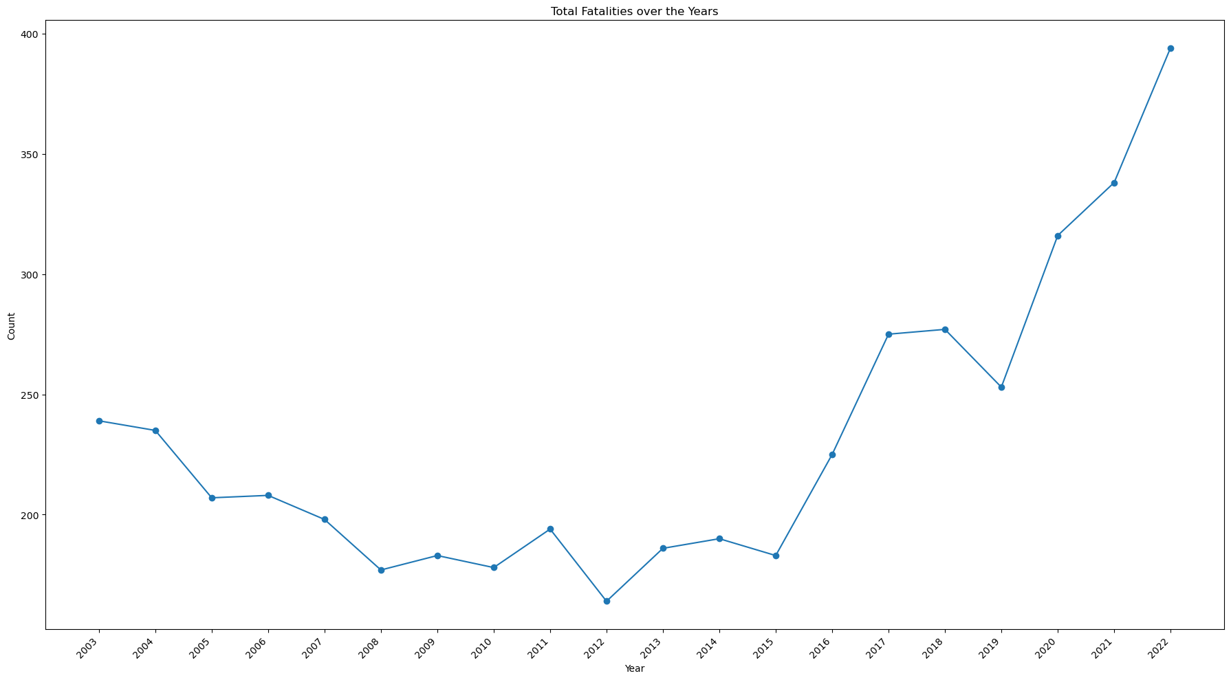
- While the number of injuries has decreased, the number of fatalities has increased, doubling from 2015 to 2022
Which products have caused the most fatalities?
Top 10 of all time
view = pd.read_sql(
'''

SELECT PRODUCT, DISP, count(CPSC_Case_Number) count
FROM neiss_prod AS prod
LEFT JOIN DispositionDim AS ddim on ddim.Code = prod.Disposition
LEFT JOIN ProductDim AS pdim on pdim.Code = prod.Product_All
WHERE Disposition = 8
GROUP BY PRODUCT
ORDER BY count DESC
LIMIT 10

'''
, neiss_conn)
view
| PRODUCT | DISP | count | |
|---|---|---|---|
| 0 | FLOORS OR FLOORING MATERIALS | 8 - FATALITY INCL. DOA, DIED IN ER | 778 |
| 1 | BEDS OR BEDFRAMES, OTHER OR NOT SPECIFIED | 8 - FATALITY INCL. DOA, DIED IN ER | 400 |
| 2 | STAIRS OR STEPS | 8 - FATALITY INCL. DOA, DIED IN ER | 325 |
| 3 | GENERAL HOME OR ROOM INVOLVEMENT IN FIRES | 8 - FATALITY INCL. DOA, DIED IN ER | 222 |
| 4 | BICYCLES AND ACCESSORIES, (EXCL.MOUNTAIN OR AL... | 8 - FATALITY INCL. DOA, DIED IN ER | 217 |
| 5 | BATHTUBS OR SHOWERS | 8 - FATALITY INCL. DOA, DIED IN ER | 155 |
| 6 | SWIMMING POOLS, NOT SPECIFIED | 8 - FATALITY INCL. DOA, DIED IN ER | 153 |
| 7 | EXERCISE (ACTIVITY OR APPAREL, W/O EQUIP) | 8 - FATALITY INCL. DOA, DIED IN ER | 122 |
| 8 | SWIMMING (ACTIVITY, APPAREL OR EQUIPMENT) | 8 - FATALITY INCL. DOA, DIED IN ER | 95 |
| 9 | SOFAS, COUCHES, DAVENPORTS, DIVANS OR STUDIO C... | 8 - FATALITY INCL. DOA, DIED IN ER | 85 |
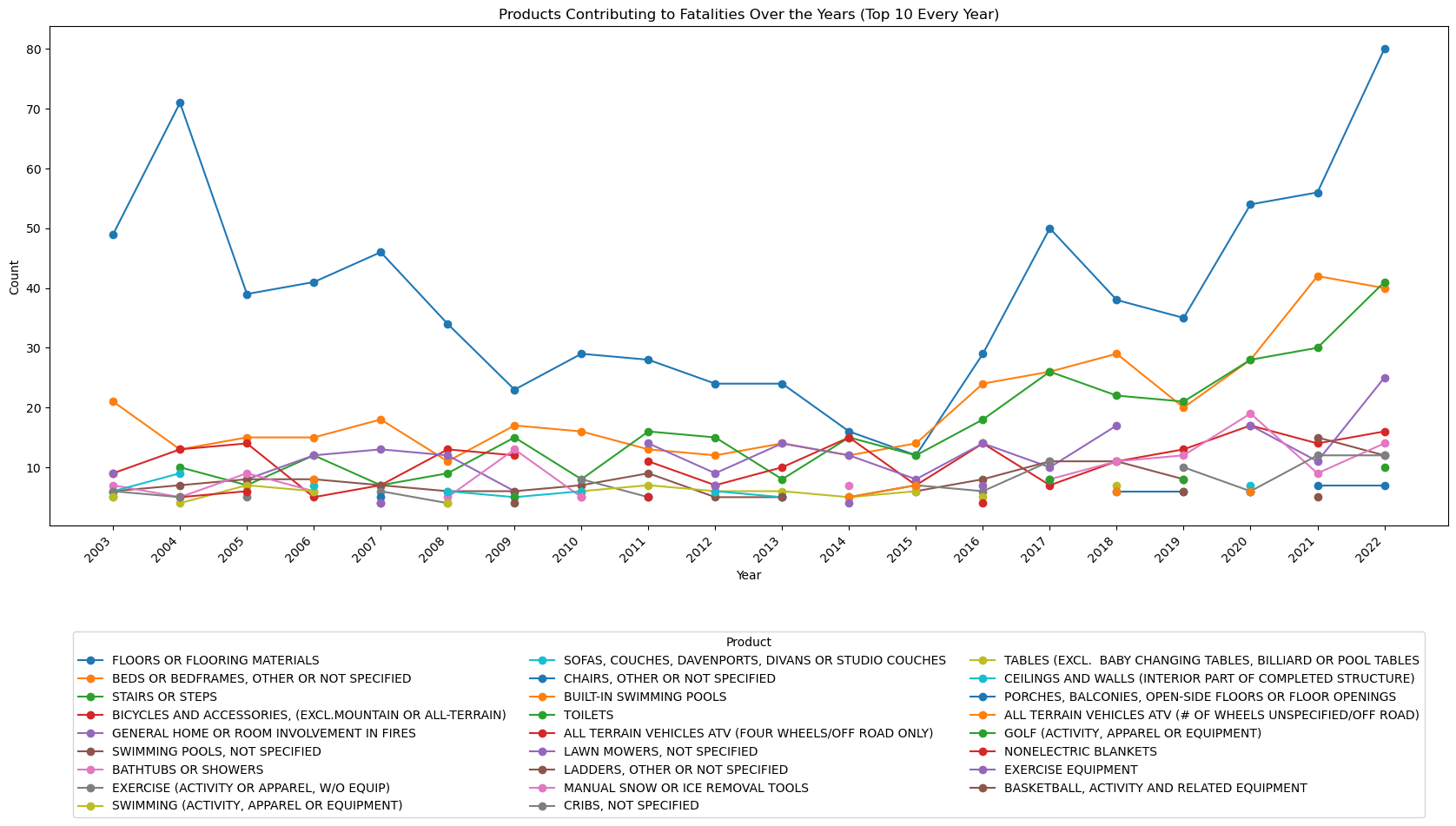
Top 10 over time
view = pd.read_sql(
'''

SELECT year, pdim.PRODUCT, count
FROM (
    SELECT year, Product_All, count(CPSC_Case_Number) as count, Disposition,
        ROW_NUMBER() OVER (PARTITION BY year ORDER BY count(CPSC_Case_Number) DESC) as rn
    FROM neiss_prod
    WHERE Disposition = 8
    GROUP BY year, Product_All
    ) subquery
LEFT JOIN ProductDim AS pdim on pdim.Code = subquery.Product_All
WHERE rn <= 10
ORDER BY year, count DESC

'''
, neiss_conn)

# Convert the 'year' column to integers
view['year'] = view['year'].astype(int)

# Pivot the data to have products as columns and years as rows
pivot_data = view.pivot(index='year', columns='PRODUCT', values='count')

# Calculate the total count for each product across all years
product_totals = pivot_data.sum().sort_values(ascending=False)

# Sort the pivot_data columns based on the product_totals order
pivot_data = pivot_data[product_totals.index]

# Plotting the line chart
fig, ax = plt.subplots(figsize=(18, 10))
pivot_data.plot(kind='line', ax=ax, marker='o')

ax.set_xlabel('Year')
ax.set_ylabel('Count')
ax.set_title('Products Contributing to Fatalities Over the Years (Top 10 Every Year)')

# Convert x-axis labels to integers and adjust rotation
ax.set_xticks(view['year'].unique())
ax.set_xticklabels(view['year'].unique(), rotation=45, ha='right')

# Move the legend below the plot
ax.legend(title='Product', bbox_to_anchor=(0.5, -0.2), loc='upper center', ncol=3)

plt.tight_layout()

plt.show()
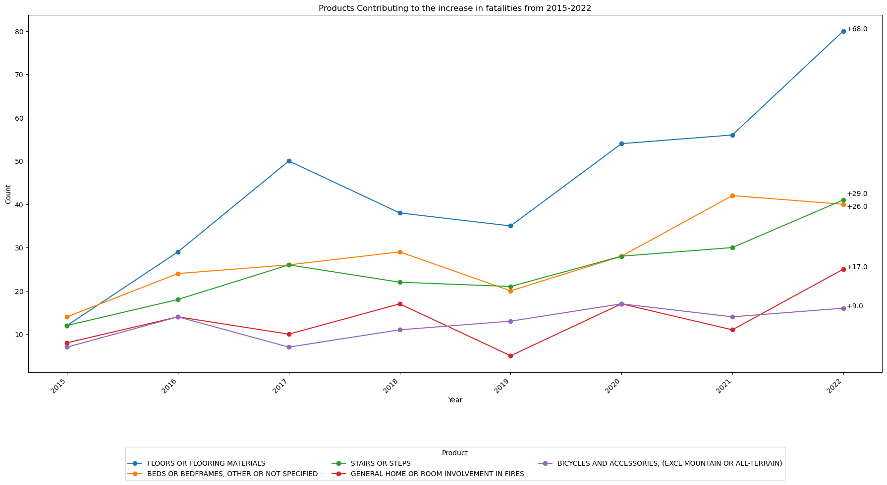
Which products are contributing most to the increase in fatalities?
view = pd.read_sql(
'''

SELECT year, pdim.PRODUCT, count(CPSC_Case_Number) count, Disposition
FROM neiss_prod
LEFT JOIN ProductDim AS pdim on pdim.Code = Product_All
WHERE year >= 2015 AND year <= 2022 AND Disposition = 8
GROUP BY Product_All, year
ORDER BY year, count DESC


'''
, neiss_conn)
This code below finds the difference between the 2015 and 2022 data and sorts according to the difference.
# Make a new dataframe that include just years 2022 and 2015
df = view[(view['year'] == 2022) | (view['year'] == 2015)]

# Pivot the table so that years 2015 and 2022 will become columns
pivot_table = df.pivot(index='PRODUCT', columns='year', values='count')
pivot_table.fillna(0,inplace=True)

# pivot_table.fillna(0, inplace=True)
pivot_table['difference'] = pivot_table[2022] - pivot_table[2015]
pivot_table = pivot_table.sort_values('difference',ascending=False)
top5 = pivot_table.nlargest(5,'difference')
top5
| year | 2015 | 2022 | difference |
|---|---|---|---|
| PRODUCT | |||
| FLOORS OR FLOORING MATERIALS | 12.0 | 80.0 | 68.0 |
| STAIRS OR STEPS | 12.0 | 41.0 | 29.0 |
| BEDS OR BEDFRAMES, OTHER OR NOT SPECIFIED | 14.0 | 40.0 | 26.0 |
| GENERAL HOME OR ROOM INVOLVEMENT IN FIRES | 8.0 | 25.0 | 17.0 |
| BICYCLES AND ACCESSORIES, (EXCL.MOUNTAIN OR ALL-TERRAIN) | 7.0 | 16.0 | 9.0 |
df = view
df = df[df['PRODUCT'].isin(top5.index)]

# Pivot the data to have products as columns and years as rows
pivot_data = df.pivot(index='year', columns='PRODUCT', values='count')

# Calculate the total count for each product across all years
product_totals = pivot_data.sum().sort_values(ascending=False)

# Sort the pivot_data columns based on the product_totals order
pivot_data = pivot_data[product_totals.index]

fig, ax = plt.subplots(figsize=(18, 10))
pivot_data.plot(kind='line', ax=ax, marker='o')

ax.set_xlabel('Year')
ax.set_ylabel('Count')
ax.set_title('Products Contributing to the increase in fatalities from 2015-2022')

# Convert x-axis labels to integers and adjust rotation
ax.set_xticks(view['year'].unique())
ax.set_xticklabels(view['year'].unique(), rotation=45, ha='right')

# Move the legend below the plot
ax.legend(title='Product', bbox_to_anchor=(0.5, -0.2), loc='upper center', ncol=3)

difference_2022 = top5['difference'].tolist()

i = 0
# Annotate the data points in 2022 with the corresponding values
for product, difference_value in zip(pivot_data.columns, difference_2022):
    i += 1
    count_2022 = pivot_data.loc[2022, product]
    if i == 2: # Adjust annotations 2 & 3 so they do not overlap
        count_2022 = count_2022 + 2
    if i == 3:
        count_2022 = count_2022 - 2
    ax.annotate("+" + f'{difference_value}', xy=(2022, count_2022), xytext=(5, 0), textcoords='offset points')


plt.tight_layout()
plt.show()
Is there any trend for people leaving without treatment?
view = pd.read_sql(
'''

SELECT year, count(CPSC_Case_Number) count
FROM neiss_all AS nall
LEFT JOIN DispositionDim AS ddim on ddim.Code = nall.Disposition
LEFT JOIN ProductDim AS pdim on pdim.Code = nall.Product_All
WHERE Disposition = 6
GROUP BY year
ORDER BY year, count DESC

'''
, neiss_conn)
# Change from view to df to avoid confusion
df = view

# Create the plot
fig, ax = plt.subplots(figsize=(18, 10))
df.sort_values('year')
df.plot(kind='line', ax=ax, marker='o', x='year',y='count', legend=False)

# Set the axis labels
ax.set_xlabel('Year')
ax.set_ylabel('Count')
ax.set_title('People leaving without treatment')

# Set the tick marks to avoid decimal numbers, set the rotation, and align the text
ax.set_xticks(view['year'].unique())
ax.set_xticklabels(view['year'].unique(), rotation=45, ha='right')


plt.tight_layout()

plt.show()
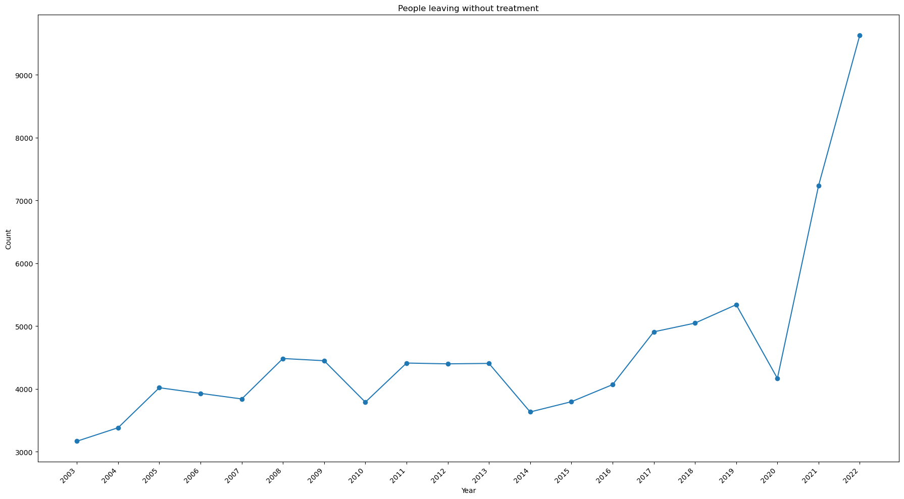
Notes:
- The number of people leaving without being seen has spiked in 2021 and 2022.
- It nearly tripled from 2020 to 2022.
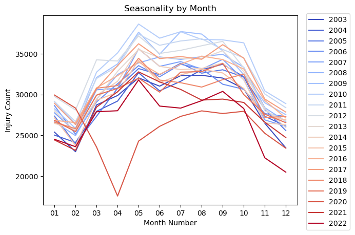
Is there a seasonality in the number of injuries?
Monthly Seasonality
view = pd.read_sql(
'''


SELECT Treatment_Date, year, strftime('%m',Treatment_Date) as month, count(CPSC_Case_Number) as count
FROM neiss_all
GROUP BY year, month


''', neiss_conn)
view
| Treatment_Date | year | month | count | |
|---|---|---|---|---|
| 0 | 2003-01-01 00:00:00 | 2003 | 01 | 25383 |
| 1 | 2003-02-01 00:00:00 | 2003 | 02 | 22992 |
| 2 | 2003-03-01 00:00:00 | 2003 | 03 | 28719 |
| 3 | 2003-04-01 00:00:00 | 2003 | 04 | 29876 |
| 4 | 2003-05-01 00:00:00 | 2003 | 05 | 32039 |
| ... | ... | ... | ... | ... |
| 235 | 2022-08-01 00:00:00 | 2022 | 08 | 29245 |
| 236 | 2022-09-01 00:00:00 | 2022 | 09 | 30385 |
| 237 | 2022-10-01 00:00:00 | 2022 | 10 | 28280 |
| 238 | 2022-11-01 00:00:00 | 2022 | 11 | 22242 |
| 239 | 2022-12-01 00:00:00 | 2022 | 12 | 20481 |
240 rows × 4 columns
import matplotlib.pyplot as plt
import numpy as np

x = df['month']
y = df['count']
z = df['year']

# Creating a colormap based on the unique values in 'z'
cmap = plt.get_cmap('coolwarm', len(np.unique(z)))

# Plotting the line chart
for i, year in enumerate(np.unique(z)):
    indices = np.where(z == year)[0]
    plt.plot(x.iloc[indices], y.iloc[indices], c=cmap(i), label=str(year))

# Moving the legend outside the chart area
plt.legend(bbox_to_anchor=(1.02, 1.03), loc='upper left')

plt.title('Seasonality by Month')
plt.xlabel('Month Number')
plt.ylabel('Injury Count')

plt.show()
This code is to confirm that the drop off was in 2020.
view[(view['year']==2020) & (view['month'] < '06')]
| Treatment_Date | year | month | count | |
|---|---|---|---|---|
| 204 | 2020-01-01 00:00:00 | 2020 | 01 | 29936 |
| 205 | 2020-02-01 00:00:00 | 2020 | 02 | 28336 |
| 206 | 2020-03-01 00:00:00 | 2020 | 03 | 23559 |
| 207 | 2020-04-01 00:00:00 | 2020 | 04 | 17554 |
| 208 | 2020-05-01 00:00:00 | 2020 | 05 | 24288 |
Notes:
- The data shows a definite seasonality over the year.
- There is an uptick in injuries over the summer months with a drop in the winter.
- February has the lowest number of injuries. It is also the shortest month of the year.
- There is a noticeable drop off in injuries in March and April of 2020. Covid 19 was declared a pandemic on March 11, 2020.
Seasonality by Day of Week
view = pd.read_sql(
'''


SELECT year, Treatment_Date, strftime('%w', Treatment_Date) as day_of_week, count(CPSC_Case_Number) as count
FROM neiss_all
GROUP BY year, day_of_week


'''
,neiss_conn)
view
| year | Treatment_Date | day_of_week | count | |
|---|---|---|---|---|
| 0 | 2003 | 2003-01-05 00:00:00 | 0 | 54811 |
| 1 | 2003 | 2003-01-06 00:00:00 | 1 | 50722 |
| 2 | 2003 | 2003-01-07 00:00:00 | 2 | 48078 |
| 3 | 2003 | 2003-01-01 00:00:00 | 3 | 47544 |
| 4 | 2003 | 2003-01-02 00:00:00 | 4 | 46273 |
| ... | ... | ... | ... | ... |
| 135 | 2022 | 2022-01-04 00:00:00 | 2 | 45332 |
| 136 | 2022 | 2022-01-05 00:00:00 | 3 | 45087 |
| 137 | 2022 | 2022-01-06 00:00:00 | 4 | 44417 |
| 138 | 2022 | 2022-01-07 00:00:00 | 5 | 44615 |
| 139 | 2022 | 2022-01-01 00:00:00 | 6 | 48034 |
140 rows × 4 columns
df = view

x = df['day_of_week']
y = df['count']
z = df['year']

# Creating a colormap based on the unique values in 'z'
cmap = plt.get_cmap('coolwarm', len(np.unique(z)))

# Plotting the line chart
for i, year in enumerate(np.unique(z)):
    indices = np.where(z == year)[0]
    plt.plot(x.iloc[indices], y.iloc[indices], c=cmap(i), label=str(year))

# Moving the legend outside the chart area
plt.legend(bbox_to_anchor=(1.02, 1.03), loc='upper left')

plt.title('Seasonality by Day of Week')
plt.xlabel('Day Number')
plt.ylabel('Injury Count')

plt.show()
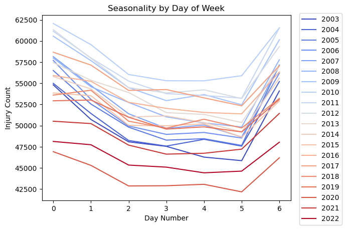
Notes:
- Sunday is represented by 0, and Saturday is represented by 6.
- As expected, there are more injuries on weekend days.
- There are more injuries on Mondays, perhaps due to the many holidays happening that day.
- Injuries drop off slightly as it gets to be later in the work week.
Seasonality by Day of Month
view = pd.read_sql(
'''


SELECT year, Treatment_Date, strftime('%d',Treatment_Date) as day_of_month, count(CPSC_Case_Number) as count
FROM neiss_all
GROUP BY year, day_of_month


'''
,neiss_conn)
view
| year | Treatment_Date | day_of_month | count | |
|---|---|---|---|---|
| 0 | 2003 | 2003-01-01 00:00:00 | 01 | 11733 |
| 1 | 2003 | 2003-01-02 00:00:00 | 02 | 11386 |
| 2 | 2003 | 2003-01-03 00:00:00 | 03 | 11346 |
| 3 | 2003 | 2003-01-04 00:00:00 | 04 | 11366 |
| 4 | 2003 | 2003-01-05 00:00:00 | 05 | 11397 |
| ... | ... | ... | ... | ... |
| 615 | 2022 | 2022-01-27 00:00:00 | 27 | 10823 |
| 616 | 2022 | 2022-01-28 00:00:00 | 28 | 10322 |
| 617 | 2022 | 2022-01-29 00:00:00 | 29 | 9877 |
| 618 | 2022 | 2022-01-30 00:00:00 | 30 | 9929 |
| 619 | 2022 | 2022-01-31 00:00:00 | 31 | 6012 |
620 rows × 4 columns
df = view

x = df['day_of_month']
y = df['count']
z = df['year']

# Creating a colormap based on the unique values in 'z'
cmap = plt.get_cmap('coolwarm', len(np.unique(z)))

# Adjust the figure size
plt.figure(figsize=(12,6))

# Plotting the line chart
for i, year in enumerate(np.unique(z)):
    indices = np.where(z == year)[0]
    plt.plot(x.iloc[indices], y.iloc[indices], c=cmap(i), label=str(year))

# Moving the legend outside the chart area
plt.legend(bbox_to_anchor=(1.02, 1.03), loc='upper left')

plt.title('Seasonality by Day of Month')
plt.xlabel('Day Number')
plt.ylabel('Injury Count')
plt.xticks(rotation=45,ha='right')


plt.show()
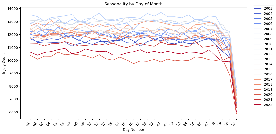
Notes:
- There is no apparent seasonality by day of month. All of the lines are fairly flat. The plot drops off at 30 and 31 probably because there are months with less than those number of days.
What body parts are most frequenty affected in injuries?
Prepare data as a View
This is another example where two columns need to be joined into one. This time a view is created instead of an actual table. Views are saved as metadata in the database file. No table is actually created. Instead, the SQL code is saved and called whenever the view is called. This saves storage space and can effectively reduce the complexity of SQL queries down the line.
# For this we have to create another table to expand the values of the two Body_Part columns. We'll create it as a view.

neiss_conn.execute(
'''

CREATE VIEW neiss_bdy AS
SELECT *
FROM
    (SELECT neiss_all.*, Body_Part as Body_Part_All
    FROM neiss_all
    WHERE Body_Part IS NOT NULL
    UNION ALL
    SELECT neiss_all.*, Body_Part_2 as Body_Part_All
    FROM neiss_all
    WHERE Body_Part_2 IS NOT NULL
    ) as subquery


'''
)
<sqlite3.Cursor at 0x7f894734bdc0>
# Confirm the data  was loaded

view = pd.read_sql(
'''

SELECT *
FROM neiss_bdy
ORDER BY Body_Part_All

'''
,neiss_conn
)

view
| index | CPSC_Case_Number | Treatment_Date | Age | Sex | Race | Other_Race | Hispanic | Body_Part | Diagnosis | ... | Product_2 | Product_3 | Narrative | Stratum | PSU | Weight | Other_Diagnosis | Other_Diagnosis_2 | year | Body_Part_All | |
|---|---|---|---|---|---|---|---|---|---|---|---|---|---|---|---|---|---|---|---|---|---|
| 0 | 203 | 90103802 | 2009-01-01 00:00:00 | 213 | 1 | 0 | None | NaN | 0 | 41 | ... | 0 | 0 | DX VOMITING: MOP CONCERNED THAT PT MAY HAVE IN... | V | 67 | 15.3491 | None | None | 2009 | 0.0 |
| 1 | 249 | 90104346 | 2009-01-02 00:00:00 | 211 | 2 | 1 | None | NaN | 0 | 41 | ... | 0 | 0 | POSSIBLY SWALLOWED PHOTOCELL BATTERY;DX INGEST... | C | 20 | 6.0260 | None | None | 2009 | 0.0 |
| 2 | 410 | 90105703 | 2009-01-03 00:00:00 | 28 | 1 | 1 | None | NaN | 0 | 41 | ... | 0 | 0 | PHARNYX FB-PIECE OF TOOTHPICK CAUGHT IN PHARNY... | V | 53 | 15.3491 | None | None | 2009 | 0.0 |
| 3 | 1015 | 90109653 | 2009-01-03 00:00:00 | 2 | 1 | 0 | None | NaN | 0 | 41 | ... | 574 | 0 | FATHER STS PT OPEN THE BACK OF A DVD REMOTE CO... | L | 50 | 62.0610 | None | None | 2009 | 0.0 |
| 4 | 1106 | 90109819 | 2009-01-02 00:00:00 | 8 | 1 | 1 | None | NaN | 0 | 41 | ... | 0 | 0 | PT.AT HOME PLAYING & SWALLOWED 2 MAGNETS FROM ... | S | 28 | 70.8387 | None | None | 2009 | 0.0 |
| ... | ... | ... | ... | ... | ... | ... | ... | ... | ... | ... | ... | ... | ... | ... | ... | ... | ... | ... | ... | ... | ... |
| 7596857 | 356194 | 200230125 | 2019-12-18 00:00:00 | 6 | 2 | 0 | None | 1.0 | 75 | 62 | ... | 0 | 0 | 6YOF P/W RINGING OF EAR AND PAIN 2/2 HAVING A ... | V | 57 | 17.3778 | None | RINGING/PAIN | 2019 | 94.0 |
| 7596858 | 357089 | 200245256 | 2019-09-22 00:00:00 | 8 | 1 | 1 | None | 1.0 | 87 | 53 | ... | 0 | 0 | 8 YOM WAS RUNNING AND FELL. MULTIPLE ABRASIONS... | C | 10 | 4.8283 | None | None | 2019 | 94.0 |
| 7596859 | 357373 | 200250688 | 2019-08-28 00:00:00 | 15 | 2 | 1 | None | 1.0 | 92 | 57 | ... | 0 | 0 | 15YOF WITH RT EAR PAIN, HAS BEEN SWIMMING A LO... | C | 10 | 4.8283 | None | SWIMMERS EAR | 2019 | 94.0 |
| 7596860 | 357523 | 200253150 | 2019-11-16 00:00:00 | 27 | 1 | 2 | None | 2.0 | 30 | 57 | ... | 0 | 0 | 27YOM FELL WHILE HAVING SEIZURE AND HIT HEAD O... | V | 64 | 16.4632 | None | None | 2019 | 94.0 |
| 7596861 | 357866 | 200255701 | 2019-11-25 00:00:00 | 77 | 2 | 1 | None | 2.0 | 75 | 59 | ... | 0 | 0 | 77YOF TRIPPED GOING UP STAIRS AT HOME AND FELL... | V | 64 | 16.4632 | None | None | 2019 | 94.0 |
7596862 rows × 30 columns
Here is a count of the two old Body_Part Columns for comparison to the row count of the new table. A subquery is used because a select statement cannot reference alias columns that were created within it. Therefore, the count of the two columns are calculated in the subquery, and then summed in the primary select statement.
view = pd.read_sql(
'''

SELECT B1, B2, B1 + B2 AS "total"
FROM (
    SELECT COUNT(Body_Part) AS B1, COUNT(Body_Part_2) AS B2
    FROM neiss_all
) AS subquery;


'''
,neiss_conn
)

view
| B1 | B2 | total | |
|---|---|---|---|
| 0 | 7316561 | 280301 | 7596862 |
The row count above and the total here match indicating that combining the columns was successful.
Analysis
view = pd.read_sql(
'''

SELECT BDYPT, count(CPSC_Case_Number) AS count
FROM neiss_bdy
LEFT JOIN BdypartDim bdy ON Code = Body_Part_All
GROUP BY BDYPT
ORDER BY count DESC

'''
,neiss_conn)
view
| BDYPT | count | |
|---|---|---|
| 0 | 75 - HEAD | 1161983 |
| 1 | 76 - FACE | 708821 |
| 2 | 92 - FINGER | 672443 |
| 3 | 79 - LOWER TRUNK | 634206 |
| 4 | 37 - ANKLE | 436942 |
| 5 | 35 - KNEE | 385366 |
| 6 | 31 - UPPER TRUNK | 376232 |
| 7 | 82 - HAND | 373804 |
| 8 | 83 - FOOT | 336107 |
| 9 | 30 - SHOULDER | 300621 |
| 10 | 33 - LOWER ARM | 287085 |
| 11 | 34 - WRIST | 264244 |
| 12 | 36 - LOWER LEG | 263319 |
| 13 | 85 - ALL PARTS BODY | 196790 |
| 14 | 32 - ELBOW | 189649 |
| 15 | 88 - MOUTH | 168696 |
| 16 | 93 - TOE | 153168 |
| 17 | 89 - NECK | 133905 |
| 18 | 77 - EYEBALL | 105146 |
| 19 | 94 - EAR | 104570 |
| 20 | 81 - UPPER LEG | 90206 |
| 21 | 80 - UPPER ARM | 81185 |
| 22 | 0 - INTERNAL | 70821 |
| 23 | 87 - NOT STATED/UNK | 64611 |
| 24 | 38 - PUBIC REGION | 35521 |
| 25 | 84 - 25-50% OF BODY | 1421 |
x = view['BDYPT']
y = view['count']
plt.figure(figsize=(15,8))
plt.bar(x,y)
plt.xticks(rotation=45, ha='right')
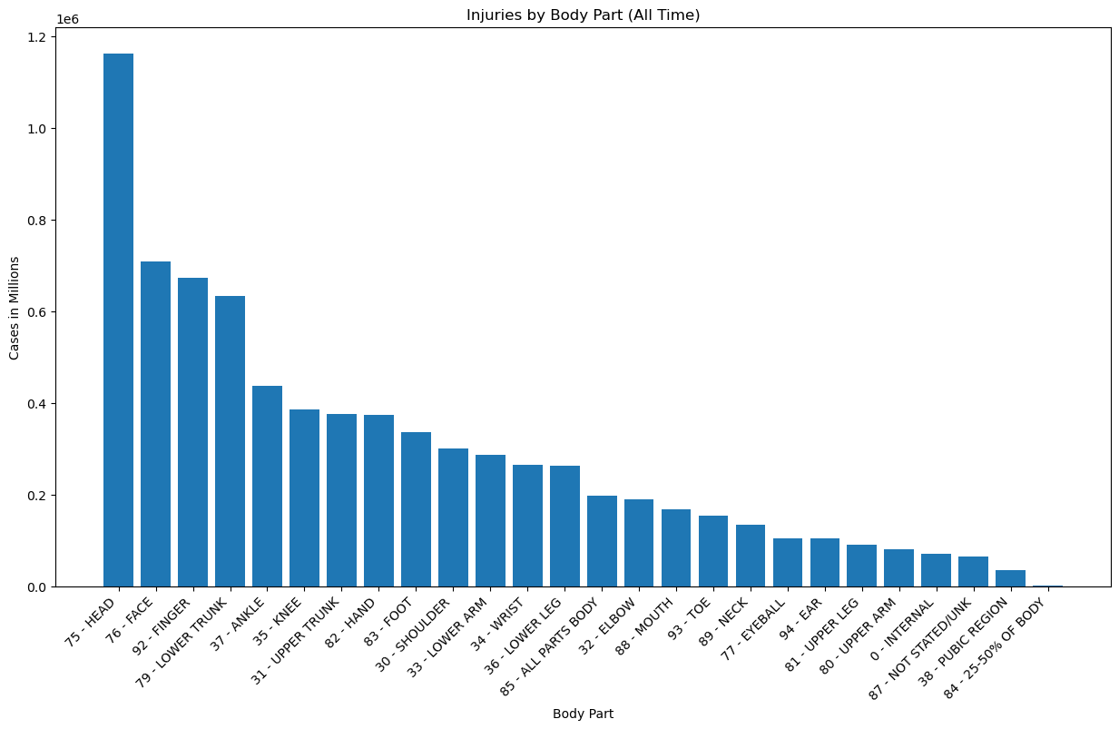
plt.title('Injuries by Body Part (All Time)')
plt.xlabel('Body Part')
plt.ylabel('Cases in Millions')
Text(0, 0.5, 'Cases in Millions')
view[view['BDYPT'].str.contains('25-50')]
| BDYPT | count | |
|---|---|---|
| 25 | 84 - 25-50% OF BODY | 1421 |
Notes:
- Most injuries are head injuries by a wide margin. Occurences were about 70% higher than the next category down.
- Face, finger, and lower trunk injuries also represented a significant portion that stood in a group of their own, about 40% above the next stage, which begins with ankle injuries at ~400k.
- Injuries that damaged 25-50% of the body were lowest, with only 1421 cases.
- It makes good sense that people would go to the hospital the most over head injuries, as they can be serious if not checked out.
- It also makes sense that finger injuries would be in the top range because they are perhaps the most prone to injury in routine activities that most people perform, such as cooking.
- Face injuries could be in the top range because people are concerned about lasting changes to their appearance, or perhaps because those injuries are particularly disturbing.
Changes Over Time
view = pd.read_sql(
'''

SELECT year, BDYPT, count, rn
FROM
    (SELECT year, Body_Part_All, count(CPSC_Case_Number) as count,
        ROW_NUMBER() OVER (PARTITION BY year ORDER BY count(CPSC_Case_Number) DESC) as rn
    FROM neiss_bdy
    GROUP BY year, Body_Part_All
) subquery
LEFT JOIN BdypartDim as bdy ON bdy.Code = subquery.Body_Part_All
ORDER BY year, count DESC

'''
,neiss_conn
)

view
| year | BDYPT | count | rn | |
|---|---|---|---|---|
| 0 | 2003 | 75 - HEAD | 40179 | 1 |
| 1 | 2003 | 92 - FINGER | 38328 | 2 |
| 2 | 2003 | 76 - FACE | 34491 | 3 |
| 3 | 2003 | 79 - LOWER TRUNK | 28871 | 4 |
| 4 | 2003 | 37 - ANKLE | 22938 | 5 |
| ... | ... | ... | ... | ... |
| 515 | 2022 | 77 - EYEBALL | 4960 | 22 |
| 516 | 2022 | 80 - UPPER ARM | 4439 | 23 |
| 517 | 2022 | 0 - INTERNAL | 4306 | 24 |
| 518 | 2022 | 38 - PUBIC REGION | 2160 | 25 |
| 519 | 2022 | 84 - 25-50% OF BODY | 15 | 26 |
520 rows × 4 columns
# Pivot the data to have products as columns and years as rows
pivot_data = view.pivot(index='year', columns='BDYPT', values='count')

# Calculate the total count for each product across all years
product_totals = pivot_data.sum().sort_values(ascending=False)

# Sort the pivot_data columns based on the product_totals order
pivot_data = pivot_data[product_totals.index]

# Plotting the line chart
fig, ax = plt.subplots(figsize=(18, 10))
pivot_data.plot(kind='line', ax=ax, marker='o')

ax.set_xlabel('Year')
ax.set_ylabel('Count')
ax.set_title('Body Part Injuries Over Time')

# Convert x-axis labels to integers and adjust rotation
ax.set_xticks(view['year'].unique())
ax.set_xticklabels(view['year'].unique(), rotation=45, ha='right')

# Move the legend below the plot
ax.legend(title='Product', bbox_to_anchor=(0.5, -0.2), loc='upper center', ncol=3)

plt.tight_layout()

plt.show()
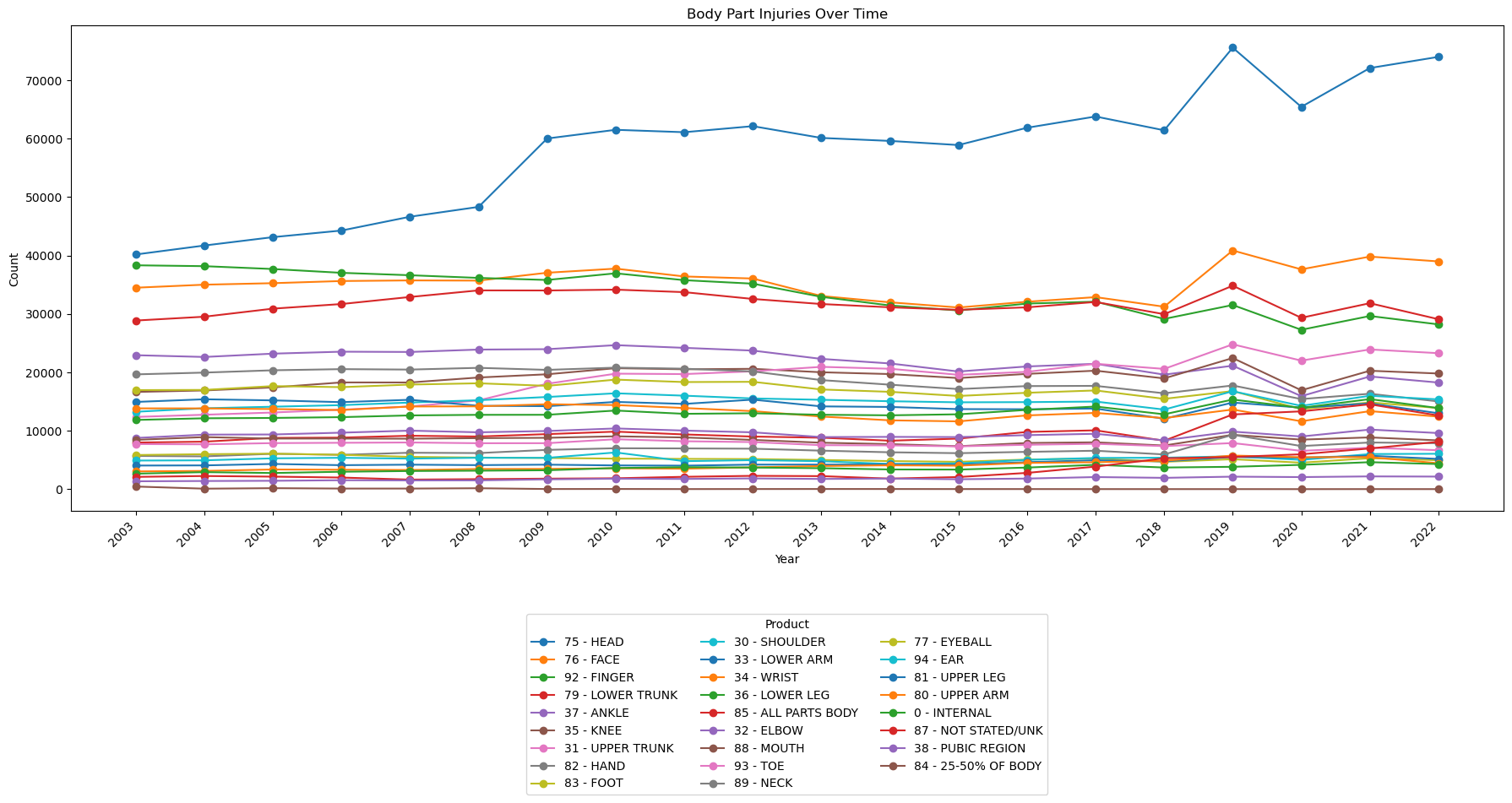
Notes:
- Head injuries have been steadily increasing since the data first became available.
- Generally, most injury categories are flat.
- There has been a noticeable uptick in head, face, and 'all parts body' injuries since 2018.
Which body part injuries are associated with the most fatalities?
view = pd.read_sql(
'''

SELECT BDYPT, Disposition, count(CPSC_Case_Number) AS count
FROM neiss_bdy
LEFT JOIN BdypartDim bdy ON bdy.Code = Body_Part_All
WHERE Disposition = 8
GROUP BY BDYPT
ORDER BY count DESC
LIMIT 15

'''
,neiss_conn)
view
| BDYPT | Disposition | count | |
|---|---|---|---|
| 0 | 85 - ALL PARTS BODY | 8 | 2539 |
| 1 | 75 - HEAD | 8 | 900 |
| 2 | 31 - UPPER TRUNK | 8 | 343 |
| 3 | 87 - NOT STATED/UNK | 8 | 235 |
| 4 | 76 - FACE | 8 | 125 |
| 5 | 79 - LOWER TRUNK | 8 | 75 |
| 6 | 89 - NECK | 8 | 67 |
| 7 | 81 - UPPER LEG | 8 | 23 |
| 8 | 36 - LOWER LEG | 8 | 21 |
| 9 | 33 - LOWER ARM | 8 | 16 |
| 10 | 0 - INTERNAL | 8 | 16 |
| 11 | 80 - UPPER ARM | 8 | 11 |
| 12 | 84 - 25-50% OF BODY | 8 | 10 |
| 13 | 35 - KNEE | 8 | 9 |
| 14 | 30 - SHOULDER | 8 | 9 |
Disposition 8 indicates fatality
x = view['BDYPT']
y = view['count']

plt.bar(x,y)
plt.xticks(rotation=45, ha='right')
plt.title('Fatalities by Body Part')
plt.xlabel('Body Part')
plt.ylabel('Cases')
Text(0, 0.5, 'Cases')
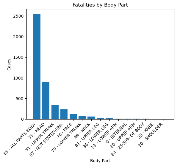
Notes:
- Injuries that involved all parts of the body had by far the most fatalities at ~2500. Could this be due to fire or explosions?
- Head injuries were second at ~900
In how many cases did 'All Parts Body' injuries involve fire?
A significant portion of fatalities fall into the All Parts Body category. The reason is explored more below.
Here the analyses begin to get more complicated, involving more variables, more joins, and multiple column concatenations.
view = pd.read_sql(
'''

SELECT BDYPT, DISP, count(CPSC_Case_Number) AS count, FIRE
FROM neiss_bdy
LEFT JOIN BdypartDim bdy ON bdy.Code = Body_Part_All
LEFT JOIN DispositionDim dis ON dis.Code = Disposition
LEFT JOIN FireDim as fire ON fire.Code = Fire_Involvement
WHERE Disposition = 8 AND BDYPT LIKE "%ALL PARTS%"
GROUP BY Fire_Involvement


'''
,neiss_conn)
view
| BDYPT | DISP | count | FIRE | |
|---|---|---|---|---|
| 0 | 85 - ALL PARTS BODY | 8 - FATALITY INCL. DOA, DIED IN ER | 2315 | NO/? |
| 1 | 85 - ALL PARTS BODY | 8 - FATALITY INCL. DOA, DIED IN ER | 197 | FD |
| 2 | 85 - ALL PARTS BODY | 8 - FATALITY INCL. DOA, DIED IN ER | 2 | NO FD |
| 3 | 85 - ALL PARTS BODY | 8 - FATALITY INCL. DOA, DIED IN ER | 25 | ? FD |
Notes:
- There were a total of 224 fatalities that involved fires
- 197 involved the fire department
- 2 did not involve the fire department
- In 25 it was unknown whether the fire department was involved
What were the diagnoses for 'All Parts Body' fatalities?
view = pd.read_sql(
'''

SELECT BDYPT, DISP, count(CPSC_Case_Number) AS count, DIAG
FROM neiss_bdy
LEFT JOIN BdypartDim bdy ON bdy.Code = Body_Part_All
LEFT JOIN DispositionDim dis ON dis.Code = Disposition
LEFT JOIN DiagnosisDim as diag ON diag.Code = Diagnosis
WHERE Disposition = 8 AND BDYPT LIKE "%ALL PARTS%"
GROUP BY Diagnosis
ORDER BY count DESC


'''
,neiss_conn)
view
| BDYPT | DISP | count | DIAG | |
|---|---|---|---|---|
| 0 | 85 - ALL PARTS BODY | 8 - FATALITY INCL. DOA, DIED IN ER | 1698 | 71 - OTHER |
| 1 | 85 - ALL PARTS BODY | 8 - FATALITY INCL. DOA, DIED IN ER | 349 | 69 - SUBMERSION |
| 2 | 85 - ALL PARTS BODY | 8 - FATALITY INCL. DOA, DIED IN ER | 276 | 65 - ANOXIA |
| 3 | 85 - ALL PARTS BODY | 8 - FATALITY INCL. DOA, DIED IN ER | 72 | 68 - POISONING |
| 4 | 85 - ALL PARTS BODY | 8 - FATALITY INCL. DOA, DIED IN ER | 58 | 51 - BURNS, THERMAL |
| 5 | 85 - ALL PARTS BODY | 8 - FATALITY INCL. DOA, DIED IN ER | 27 | 62 - INTERNAL INJURY |
| 6 | 85 - ALL PARTS BODY | 8 - FATALITY INCL. DOA, DIED IN ER | 17 | 67 - ELECTRIC SHOCK |
| 7 | 85 - ALL PARTS BODY | 8 - FATALITY INCL. DOA, DIED IN ER | 10 | 57 - FRACTURE |
| 8 | 85 - ALL PARTS BODY | 8 - FATALITY INCL. DOA, DIED IN ER | 10 | 53 - CONTUSIONS, ABR. |
| 9 | 85 - ALL PARTS BODY | 8 - FATALITY INCL. DOA, DIED IN ER | 8 | 59 - LACERATION |
| 10 | 85 - ALL PARTS BODY | 8 - FATALITY INCL. DOA, DIED IN ER | 3 | 58 - HEMATOMA |
| 11 | 85 - ALL PARTS BODY | 8 - FATALITY INCL. DOA, DIED IN ER | 2 | 66 - HEMORRHAGE |
| 12 | 85 - ALL PARTS BODY | 8 - FATALITY INCL. DOA, DIED IN ER | 2 | 54 - CRUSHING |
| 13 | 85 - ALL PARTS BODY | 8 - FATALITY INCL. DOA, DIED IN ER | 2 | 47 - BURN, NOT SPEC. |
| 14 | 85 - ALL PARTS BODY | 8 - FATALITY INCL. DOA, DIED IN ER | 1 | 72 - AVULSION |
| 15 | 85 - ALL PARTS BODY | 8 - FATALITY INCL. DOA, DIED IN ER | 1 | 63 - PUNCTURE |
| 16 | 85 - ALL PARTS BODY | 8 - FATALITY INCL. DOA, DIED IN ER | 1 | 56 - FOREIGN BODY |
| 17 | 85 - ALL PARTS BODY | 8 - FATALITY INCL. DOA, DIED IN ER | 1 | 48 - BURN, SCALD |
| 18 | 85 - ALL PARTS BODY | 8 - FATALITY INCL. DOA, DIED IN ER | 1 | 46 - BURN, ELECTRICAL |
Notes:
- Drowning was the number one cause of death at 349. We will have to dig into the other diagnoses to get more information.
- Anoxia, which is a lack of oxygen, was number two at 276.
- Poisoning was number three at 72.
- Burns was a relatively close four at 58.
- There is a significant portion listed as 'Other'
What additional diagnoses are there?
view = pd.read_sql(
'''

SELECT BDYPT, DISP, count(CPSC_Case_Number) AS count, DIAG, Other_Diagnosis, Other_Diagnosis_2
FROM neiss_bdy
LEFT JOIN BdypartDim bdy ON bdy.Code = Body_Part_All
LEFT JOIN DispositionDim dis ON dis.Code = Disposition
LEFT JOIN DiagnosisDim as diag ON diag.Code = Diagnosis
WHERE Disposition = 8 AND BDYPT LIKE "%ALL PARTS%" AND DIAG = "71 - OTHER"
GROUP BY Other_Diagnosis
ORDER BY count DESC


'''
,neiss_conn)
view
| BDYPT | DISP | count | DIAG | Other_Diagnosis | Other_Diagnosis_2 | |
|---|---|---|---|---|---|---|
| 0 | 85 - ALL PARTS BODY | 8 - FATALITY INCL. DOA, DIED IN ER | 745 | 71 - OTHER | None | None |
| 1 | 85 - ALL PARTS BODY | 8 - FATALITY INCL. DOA, DIED IN ER | 719 | 71 - OTHER | CARDIAC ARREST | None |
| 2 | 85 - ALL PARTS BODY | 8 - FATALITY INCL. DOA, DIED IN ER | 17 | 71 - OTHER | CARDIOPULMONARY ARREST | None |
| 3 | 85 - ALL PARTS BODY | 8 - FATALITY INCL. DOA, DIED IN ER | 15 | 71 - OTHER | TRAUMATIC ARREST | None |
| 4 | 85 - ALL PARTS BODY | 8 - FATALITY INCL. DOA, DIED IN ER | 13 | 71 - OTHER | TRAUMATIC CARDIAC ARREST | None |
| ... | ... | ... | ... | ... | ... | ... |
| 113 | 85 - ALL PARTS BODY | 8 - FATALITY INCL. DOA, DIED IN ER | 1 | 71 - OTHER | ARREST, CARDIO | None |
| 114 | 85 - ALL PARTS BODY | 8 - FATALITY INCL. DOA, DIED IN ER | 1 | 71 - OTHER | ARDIAC ARREST | None |
| 115 | 85 - ALL PARTS BODY | 8 - FATALITY INCL. DOA, DIED IN ER | 1 | 71 - OTHER | AMS | None |
| 116 | 85 - ALL PARTS BODY | 8 - FATALITY INCL. DOA, DIED IN ER | 1 | 71 - OTHER | ACUTE RESPIRATORY FAILURE | None |
| 117 | 85 - ALL PARTS BODY | 8 - FATALITY INCL. DOA, DIED IN ER | 1 | 71 - OTHER | ACUTE RENAL FAILURE | MYOCARDIAL INFARCTION |
118 rows × 6 columns
Notes:
- It appears that heart attacks and organ failures are a primary reason that injuries are classified as 'All Parts Body'
What was the percentage of injuries that involved alcohol or drugs?
In this code, two subqueries are created, one to the individual counts for the Alcohol and Drug columns, and another to calculate the total account of all of the rows where those two columns are not null. This is done because these columns were not included until 2019, hence all of the data for the cells prior to those years is marked as null.
The percentage calculation is done in the primary select statement.
view = pd.read_sql(
'''

SELECT count, Fire_Involvement, Alcohol, Drug, (CAST(count AS FLOAT) * 100 / total_count) as percentage
FROM
    (SELECT count(CPSC_Case_Number) AS count, Fire_Involvement, Alcohol, Drug
    FROM neiss_all
    WHERE Alcohol IS NOT NULL AND DRUG IS NOT NULL
    GROUP BY  Alcohol, Drug) subquery,
    (SELECT COUNT(*) AS total_count
    FROM neiss_all
    WHERE Alcohol IS NOT NULL AND DRUG IS NOT NULL) total_rows


'''
,neiss_conn)
view
| count | Fire_Involvement | Alcohol | Drug | percentage | |
|---|---|---|---|---|---|
| 0 | 1281432 | 0 | 0.0 | 0.0 | 96.212994 |
| 1 | 24799 | 0 | 0.0 | 1.0 | 1.861969 |
| 2 | 23317 | 0 | 1.0 | 0.0 | 1.750696 |
| 3 | 2322 | 0 | 1.0 | 1.0 | 0.174341 |
- Less than 4% of injuries from 2019 to 2022 involved alcohol or drugs
- The data in this case is truncated to not include the null values because recording of this data did not begin until 2019.
What age group is most suceptible to injury?
In this code, there are several ages coded 201 to 223 that represent ages in months for children aged 0-1. The SQL code below changes those values so that they will be represented as 0 or 1 in this analysis. Values that were originally 0 represent ages that were unknown at the time of recording. They are changed to NULL so that they won't be included in the distribution plot.
View = pd.read_sql(
'''

SELECT Age, CASE
    WHEN Age = 0 THEN NULL
    WHEN Age BETWEEN 200 AND 211 THEN 0
    WHEN Age BETWEEN 212 AND 223 THEN 1
    ELSE Age
    END AS AgeInc
FROM neiss_all
ORDER BY AgeInc


'''
,neiss_conn)
View
| Age | AgeInc | |
|---|---|---|
| 0 | 0 | NaN |
| 1 | 0 | NaN |
| 2 | 0 | NaN |
| 3 | 0 | NaN |
| 4 | 0 | NaN |
| ... | ... | ... |
| 7316556 | 112 | 112.0 |
| 7316557 | 112 | 112.0 |
| 7316558 | 113 | 113.0 |
| 7316559 | 113 | 113.0 |
| 7316560 | 113 | 113.0 |
7316561 rows × 2 columns
Check to make sure that 0, 1, and null are included
View['AgeInc'].unique()
array([ nan,   0.,   1.,   2.,   3.,   4.,   5.,   6.,   7.,   8.,   9.,
        10.,  11.,  12.,  13.,  14.,  15.,  16.,  17.,  18.,  19.,  20.,
        21.,  22.,  23.,  24.,  25.,  26.,  27.,  28.,  29.,  30.,  31.,
        32.,  33.,  34.,  35.,  36.,  37.,  38.,  39.,  40.,  41.,  42.,
        43.,  44.,  45.,  46.,  47.,  48.,  49.,  50.,  51.,  52.,  53.,
        54.,  55.,  56.,  57.,  58.,  59.,  60.,  61.,  62.,  63.,  64.,
        65.,  66.,  67.,  68.,  69.,  70.,  71.,  72.,  73.,  74.,  75.,
        76.,  77.,  78.,  79.,  80.,  81.,  82.,  83.,  84.,  85.,  86.,
        87.,  88.,  89.,  90.,  91.,  92.,  93.,  94.,  95.,  96.,  97.,
        98.,  99., 100., 101., 102., 103., 104., 105., 106., 107., 108.,
       109., 110., 111., 112., 113.])
g = sns.displot(View['AgeInc'], kde=True)
# kde=True combines the line with the columns
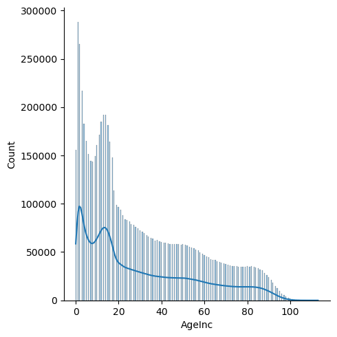
Notes:
- Younger age groups (<20) are significantly more susceptible to injury
- There is a dip that occurs at the ages of 5-9. Injuries peak at about 192k at the ages of 13 and 14, and then steadily decrease from there.
- Injuries pick up a bit in the early 50s, and again in the 80s.
What is the injury distribution for children under two years?
This code removes all ages accept for those under two years. 200 is subtracted from the number code to get the corresponding age in months
view = pd.read_sql(
'''

SELECT Age, CASE
    WHEN AGE BETWEEN 201 AND 223 THEN AGE - 200
    ELSE AGE = NULL
    END AS age_months
FROM neiss_all
WHERE age_months IS NOT NULL
ORDER BY age_months

'''
,neiss_conn)
view
| Age | age_months | |
|---|---|---|
| 0 | 201 | 1 |
| 1 | 201 | 1 |
| 2 | 201 | 1 |
| 3 | 201 | 1 |
| 4 | 201 | 1 |
| ... | ... | ... |
| 443944 | 223 | 23 |
| 443945 | 223 | 23 |
| 443946 | 223 | 23 |
| 443947 | 223 | 23 |
| 443948 | 223 | 23 |
443949 rows × 2 columns
g = sns.displot(view['age_months'], kde=True)
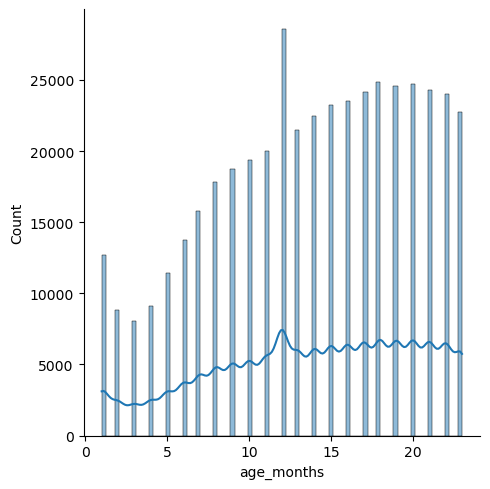
Notes:
- The distribution steadily increases with an increase in age.
- The peak in the beginning could be explained by parents not being used to handling babies, or perhaps because they are more vulnerable at that age.
- The steady increase from 3 months on could be due to children learning how to walk, and therefore being prone to more accidents.
- The spike at 12 months is likely due to erroneous input--perhaps personnel inputting 12 months because they have forgotten what age the baby was.
Where did most injuries happen?
view = pd.read_sql(
'''

SELECT LOC, count(CPSC_Case_Number) as count
FROM neiss_all
LEFT JOIN LocationDim AS loc ON loc.Code = Location
GROUP BY LOC
ORDER BY count DESC

'''
,neiss_conn)
view
| LOC | count | |
|---|---|---|
| 0 | HOME | 3352026 |
| 1 | UNK | 2016290 |
| 2 | SPORTS | 916225 |
| 3 | PUBLIC | 464726 |
| 4 | SCHOOL | 382237 |
| 5 | STREET | 178503 |
| 6 | FARM | 4160 |
| 7 | MOBILE | 1855 |
| 8 | INDST. | 539 |
x = view['LOC']
y = view['count']
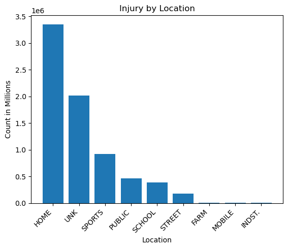
plt.bar(x,y)
plt.title('Injury by Location')
plt.xlabel('Location')
plt.ylabel('Count in Millions')
plt.xticks(rotation=45,ha='right')
plt.plot()
[]
v = view[view['LOC']=='HOME'].iloc[0].values
x = view[view['LOC']=='SPORTS'].iloc[0].values
z = view[(view['LOC']!='HOME') & (view['LOC']!='UNK')].sum()
print('Home/All: ',(v[1]/ z[1]))
print('Home/Sports: ',(v[1]/ x[1]))
Home/All:  1.720536174865071
Home/Sports:  3.6585183770362084
Notes:
- Most injuries happened at home.
- Home had 3.7 times the number of sports injuries, and 1.72 times the number of all other locations combined, not including those labelled as unknown.
- Industrial, farm, and mobile injuries were very low by comparison.
What was the most commmon diagnosis?
Prepare the data
# Create a view to combine the two diagnosis columns

neiss_conn.execute(
'''

CREATE VIEW neiss_diag AS
    SELECT *
        FROM
            (SELECT neiss_all.*, Diagnosis as Diagnosis_All
            FROM neiss_all
            WHERE Diagnosis IS NOT NULL
            UNION ALL
            SELECT neiss_all.*, Diagnosis_2 as Diagnosis_All
            FROM neiss_all
            WHERE Diagnosis_2 IS NOT NULL)
    ORDER BY Treatment_Date

'''
)
<sqlite3.Cursor at 0x7f8ad5c674c0>
Another count of the rows to compare to the resulting table.
view = pd.read_sql(
'''

SELECT C1, C2, C1 + C2 as Total
    FROM (SELECT count(Diagnosis) as C1, count(Diagnosis_2) as C2
            FROM neiss_all)

'''
, neiss_conn)
view
| C1 | C2 | Total | |
|---|---|---|---|
| 0 | 7316561 | 280301 | 7596862 |
view = pd.read_sql(
'''

SELECT *
FROM neiss_diag

'''
, neiss_conn)
view
| index | CPSC_Case_Number | Treatment_Date | Age | Sex | Race | Other_Race | Hispanic | Body_Part | Diagnosis | ... | Product_2 | Product_3 | Narrative | Stratum | PSU | Weight | Other_Diagnosis | Other_Diagnosis_2 | year | Diagnosis_All | |
|---|---|---|---|---|---|---|---|---|---|---|---|---|---|---|---|---|---|---|---|---|---|
| 0 | 0 | 30102578 | 2003-01-01 00:00:00 | 33 | 1 | 1 | None | NaN | 30 | 57 | ... | 0 | 0 | 33 YOWM WRECKED HIS 4-WHEELER ANS INJURED HIS ... | S | 1 | 71.3643 | None | None | 2003 | 57.0 |
| 1 | 1 | 30102580 | 2003-01-01 00:00:00 | 3 | 1 | 1 | None | NaN | 75 | 53 | ... | 0 | 0 | 3 YOWM FELL DOWN APPROX 3-4 WOODEN STEPS AND I... | S | 1 | 71.3643 | None | None | 2003 | 53.0 |
| 2 | 2 | 30102586 | 2003-01-01 00:00:00 | 37 | 1 | 1 | None | NaN | 83 | 53 | ... | 0 | 0 | 37 YOWM SUSTAINED AN ABRASION TO HIS FOOT FROM... | S | 1 | 71.3643 | None | None | 2003 | 53.0 |
| 3 | 9 | 30102625 | 2003-01-01 00:00:00 | 43 | 1 | 2 | None | NaN | 79 | 64 | ... | 0 | 0 | PT. WAS FOUND ON FLOOR AND COULDN'T GET UP, ET... | M | 14 | 42.4038 | None | None | 2003 | 64.0 |
| 4 | 10 | 30102626 | 2003-01-01 00:00:00 | 51 | 2 | 2 | None | NaN | 35 | 64 | ... | 0 | 0 | FELL DUE TO WET KITCHEN FLOOR AT HOME, LANDED ... | M | 14 | 42.4038 | None | None | 2003 | 64.0 |
| ... | ... | ... | ... | ... | ... | ... | ... | ... | ... | ... | ... | ... | ... | ... | ... | ... | ... | ... | ... | ... | ... |
| 7596857 | 323081 | 230235679 | 2022-12-31 00:00:00 | 15 | 1 | 1 | None | 2.0 | 83 | 53 | ... | 0 | 0 | 15YOM PRESENTS WITH LEFT FOOT INJURY WHEN HE L... | C | 8 | 7.7789 | None | None | 2022 | 64.0 |
| 7596858 | 323083 | 230235681 | 2022-12-31 00:00:00 | 8 | 1 | 2 | None | 2.0 | 88 | 60 | ... | 0 | 0 | 8YOM PRESENTS WITH DENTAL INJURY AFTER FALLING... | C | 8 | 7.7789 | None | None | 2022 | 66.0 |
| 7596859 | 323084 | 230235682 | 2022-12-31 00:00:00 | 7 | 2 | 1 | None | 2.0 | 88 | 60 | ... | 0 | 0 | 7YOF WAS RIDING A HOVERBOARD WHEN SHE FELL, WA... | C | 8 | 7.7789 | None | PAIN | 2022 | 71.0 |
| 7596860 | 323094 | 230235695 | 2022-12-31 00:00:00 | 212 | 1 | 3 | MULTI-RACIAL | 0.0 | 75 | 62 | ... | 1807 | 0 | 12MOM FELL DOWN 15 HARDWOOD STAIRS ONTO HARDWO... | C | 8 | 7.7789 | None | None | 2022 | 59.0 |
| 7596861 | 323095 | 230235696 | 2022-12-31 00:00:00 | 8 | 1 | 1 | None | 2.0 | 75 | 62 | ... | 1884 | 0 | 8YOM WAS PLAYING A VIRTUAL REALITY GAME WHEN H... | C | 8 | 7.7789 | None | None | 2022 | 59.0 |
7596862 rows × 30 columns
The row number matches with the expected results from the prior code.
Top Diagnoses of all time
view = pd.read_sql(
'''

SELECT DIAG, count(CPSC_Case_Number) as count
FROM neiss_diag
LEFT JOIN DiagnosisDim ON Code = Diagnosis_All
GROUP BY DIAG
ORDER BY count DESC


'''
, neiss_conn)
view
| DIAG | count | |
|---|---|---|
| 0 | 59 - LACERATION | 1439873 |
| 1 | 53 - CONTUSIONS, ABR. | 1169958 |
| 2 | 57 - FRACTURE | 1168267 |
| 3 | 64 - STRAIN, SPRAIN | 1112022 |
| 4 | 71 - OTHER | 949588 |
| 5 | 62 - INTERNAL INJURY | 660834 |
| 6 | 56 - FOREIGN BODY | 145340 |
| 7 | 52 - CONCUSSION | 140794 |
| 8 | 55 - DISLOCATION | 116689 |
| 9 | 68 - POISONING | 102446 |
| 10 | 58 - HEMATOMA | 78456 |
| 11 | 63 - PUNCTURE | 78146 |
| 12 | 51 - BURNS, THERMAL | 68249 |
| 13 | 41 - INGESTION | 60361 |
| 14 | 48 - BURN, SCALD | 49086 |
| 15 | 72 - AVULSION | 47596 |
| 16 | 74 - DERMA/CONJUNCT | 45571 |
| 17 | 60 - DENTAL INJURY | 39706 |
| 18 | 65 - ANOXIA | 20768 |
| 19 | 61 - NERVE DAMAGE | 19351 |
| 20 | 54 - CRUSHING | 16633 |
| 21 | 50 - AMPUTATION | 14962 |
| 22 | 66 - HEMORRHAGE | 13464 |
| 23 | 42 - ASPIRATION | 10454 |
| 24 | 49 - BURN, CHEMICAL | 10222 |
| 25 | 69 - SUBMERSION | 6304 |
| 26 | 73 - RADIATION | 4547 |
| 27 | 67 - ELECTRIC SHOCK | 3594 |
| 28 | 46 - BURN, ELECTRICAL | 2361 |
| 29 | 47 - BURN, NOT SPEC. | 1220 |
x = view['DIAG']
y = view['count']
plt.figure(figsize=(10,6))
plt.bar(x,y)
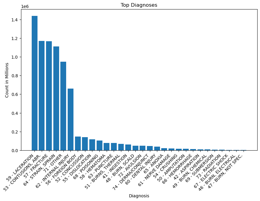
plt.title('Top Diagnoses')
plt.xlabel('Diagnosis')
plt.ylabel('Count in Millions')
plt.xticks(rotation=45,ha='right')
plt.plot()
[]
a = view[view['DIAG'].str.contains('59 - LAC')].iloc[0].values
a = a[1]
b = view[view['DIAG'].str.contains('62 - INT')].iloc[0].values
b = b[1]
print('LAC = ',a)
print('INT = ',b)
print('LAC / INT = ',a/b)
LAC =  1439873
INT =  660834
LAC / INT =  2.1788724551097554
Notes:
- The top diagnoses in order were, lacerations, contusions, fractures, strains/sprains, and internal injuries (ignoring other). These diagnoses stood in a group of their own above the remaining diagnoses, which included foreign body, concussion, dislocation, and poisoning.
- Lacerations are cuts or tears in the skin, while contusions are bruises. Internal injuries, unlike contusions, are not visible on the surface of the skin. They involve structural damage to internal organs or blood vessels.
- Internal injuries are 660,834. The number is about half of laceration injuries, which is at 1,439,873.
What products are involved in laceration injuries?
In this code below, we are stacking the three product columns on top of the two stacked diagnosis columns. We have to be careful for erroneous numbers here because entries are duplicated when the columns are stacked. In this case, it is not an issue, for one, because we are filtering by one diagnosis. There will not be cases where one diagnosis was repeated in both diagnosis columns. However, we must be aware that we are looking at duplicated cases for the product columns across the different products. This means that we are not looking at number of cases, but number of instances where the given product was involved. This is has indeed been the case for all of the supplementary tables and views we have created thus far (neiss_prod, neiss_bdy, etc). If we were to aggregate the total count, we would get a number that is higher than the actual number of cases. This is reflected in the fact that as we've been checking our views, we have been getting row numbers that are higher than the original total case number of 7,316,561.
Even if we decide to use just the first column (as was done in one case earlier), we still get a good idea of the underlying data because the first column is always fully populated, while the supplementary columns contain only a small fraction of data in comparison.
view = pd.read_sql(
'''

SELECT DIAG, PRODUCT, count(CPSC_Case_Number) as count
FROM (
    SELECT neiss_diag.*, product_1 AS Product_All
    FROM neiss_diag
    WHERE Product_1 != 0
    UNION ALL
    SELECT neiss_diag.*, product_2 AS Product_All
    FROM neiss_diag
    WHERE Product_2 != 0
    UNION ALL
    SELECT neiss_diag.*, product_3 AS Product_All
    FROM neiss_diag
    WHERE Product_3 != 0
) AS Subquery
LEFT JOIN DiagnosisDim AS diag ON diag.Code = Diagnosis_All
LEFT JOIN ProductDim AS prod ON prod.Code = Product_1
WHERE DIAG LIKE "%LACERATION%"
GROUP BY DIAG, Product_All
ORDER BY count DESC
LIMIT 20


'''
,neiss_conn
)
view
| DIAG | PRODUCT | count | |
|---|---|---|---|
| 0 | 59 - LACERATION | KNIVES, NOT ELSEWHERE CLASSIFIED | 154591 |
| 1 | 59 - LACERATION | FLOORS OR FLOORING MATERIALS | 92291 |
| 2 | 59 - LACERATION | TABLES (EXCL. BABY CHANGING TABLES, BILLIARD ... | 86958 |
| 3 | 59 - LACERATION | BEDS OR BEDFRAMES, OTHER OR NOT SPECIFIED | 66201 |
| 4 | 59 - LACERATION | STAIRS OR STEPS | 58037 |
| 5 | 59 - LACERATION | BICYCLES AND ACCESSORIES, (EXCL.MOUNTAIN OR AL... | 49901 |
| 6 | 59 - LACERATION | DOORS, OTHER OR NOT SPECIFIED | 43999 |
| 7 | 59 - LACERATION | CEILINGS AND WALLS (INTERIOR PART OF COMPLETED... | 39148 |
| 8 | 59 - LACERATION | WINDOWS AND WINDOW GLASS, OTHER THAN STORM WIN... | 38054 |
| 9 | 59 - LACERATION | CHAIRS, OTHER OR NOT SPECIFIED | 37936 |
| 10 | 59 - LACERATION | DRINKING GLASSES, CUPS, AND MUGS | 31805 |
| 11 | 59 - LACERATION | CABINETS, RACKS, ROOM DIVIDERS AND SHELVES, NEC | 31524 |
| 12 | 59 - LACERATION | TABLEWARE AND ACCESSORIES | 29780 |
| 13 | 59 - LACERATION | BATHTUBS OR SHOWERS | 28466 |
| 14 | 59 - LACERATION | METAL CONTAINERS | 26212 |
| 15 | 59 - LACERATION | BASKETBALL, ACTIVITY AND RELATED EQUIPMENT | 24782 |
| 16 | 59 - LACERATION | FENCES OR FENCE POSTS | 24112 |
| 17 | 59 - LACERATION | DESKS, CHESTS, BUREAUS OR BUFFETS | 21967 |
| 18 | 59 - LACERATION | KNIVES WITH REPLACEABLE BLADES | 20791 |
| 19 | 59 - LACERATION | SOFAS, COUCHES, DAVENPORTS, DIVANS OR STUDIO C... | 18138 |
Notes:
- Perhaps not surprisingly, knives are the number one cause of lacerations.
- More surpsisingly, tables are number three, perhaps from people falling into them.
- Floors and stairs are once again near the top of the list.
Text Analysis
A narrative column is included in the table so that we might glean additional insights. We'll keep it simple with some word frequency analysis.
Why did so many cases involve beds?
Considering beds are primarily used for sedentary activities, it is interesting that they were involved in so many injuries. This subsection explores this reasoning further.
Was moving involved?
# Change the settings for pandas so the entire contents of the cell can be viewed.

pd.set_option('display.max_colwidth', None)
In this code, we are essentially combining two tables into one. In table one, which is created in the subquery before the UNION ALL statement, we are creating a count for all of the cases that involved products with 'BED ' in the product name. In table two, we are creating a count for all of those same product names, but that also contain ' move ' or ' moving ' in the narrative column. Here are some important notes regarding the code:
- UNION ALL combines columns based on order and not alias name. Therefore, the columns in the select statements for each table in the subquery must be specified in the order they are to be combined in.
- The SUM() methods must be used in the main select statement so that the counts will be aggregated properly.
- CAST is used in the Percentage column because C1 and C2 are both integers. Casting them as floats assures that there won't be issues with bounds or rounding.
- Logical statements are separated into parentheses groups to keep the logic clear.
- Spaces are included in the keywords to keep words like 'movement' out of the results.
view = pd.read_sql(
'''

SELECT PRODUCT, SUM(C2) as Parts_with_Text, SUM(C1) as Total, 100*CAST(SUM(C2) AS FLOAT)/CAST(SUM(C1) AS FLOAT) as Percentage
    FROM
    (SELECT PRODUCT, count(CPSC_Case_Number) as C1, 0 as C2, Narrative
    FROM neiss_prod as neiss
    LEFT JOIN ProductDim AS prod ON prod.Code = neiss.Product_All
    WHERE PRODUCT LIKE "%BEDS %"
    GROUP BY PRODUCT

    UNION ALL

    SELECT PRODUCT, 0 as C1, count(CPSC_Case_Number) as C2, Narrative
    FROM neiss_prod as neiss
    LEFT JOIN ProductDim AS prod ON prod.Code = neiss.Product_All
    WHERE (PRODUCT LIKE "%BEDS %")
    AND (Narrative LIKE "% MOVE %" OR Narrative LIKE "% MOVING %")
    GROUP BY PRODUCT) sub
GROUP BY PRODUCT
ORDER BY Total DESC


'''
,neiss_conn
)
view
| PRODUCT | Parts_with_Text | Total | Percentage | |
|---|---|---|---|---|
| 0 | BEDS OR BEDFRAMES, OTHER OR NOT SPECIFIED | 4002 | 365585 | 1.094684 |
| 1 | CONVERTIBLE BEDS, HIDEAWAY BEDS OR SOFA BEDS | 120 | 903 | 13.289037 |
| 2 | WATERBEDS OR WATER PILLOWS | 22 | 229 | 9.606987 |
Notes:
- Only a small percentage of the cases involved moving.
- Convertible bed injuries likely more frequently involved the key phrases because they involve moving parts by design.
Were people falling from the beds?
view = pd.read_sql(
'''

SELECT PRODUCT, SUM(C2) as Parts_with_Text, SUM(C1) as Total, 100*CAST(SUM(C2) AS FLOAT)/CAST(SUM(C1) AS FLOAT) as Percentage
    FROM
    (SELECT PRODUCT, count(CPSC_Case_Number) as C1, 0 as C2, Narrative
    FROM neiss_prod as neiss
    LEFT JOIN ProductDim AS prod ON prod.Code = neiss.Product_All
    WHERE PRODUCT LIKE "%BEDS %"
    GROUP BY PRODUCT

    UNION ALL

    SELECT PRODUCT, 0 as C1, count(CPSC_Case_Number) as C2, Narrative
    FROM neiss_prod as neiss
    LEFT JOIN ProductDim AS prod ON prod.Code = neiss.Product_All
    WHERE (PRODUCT LIKE "%BEDS %")
    AND (Narrative LIKE "%FELL%" OR Narrative LIKE "%FALL%")
    GROUP BY PRODUCT) sub
GROUP BY PRODUCT
ORDER BY Total DESC


'''
,neiss_conn
)
view
| PRODUCT | Parts_with_Text | Total | Percentage | |
|---|---|---|---|---|
| 0 | BEDS OR BEDFRAMES, OTHER OR NOT SPECIFIED | 245796 | 365585 | 67.233612 |
| 1 | CONVERTIBLE BEDS, HIDEAWAY BEDS OR SOFA BEDS | 239 | 903 | 26.467331 |
| 2 | WATERBEDS OR WATER PILLOWS | 89 | 229 | 38.864629 |
Notes:
- Falling was involved much more frequently than moving.
- 67% of cases for the main bed category involved falling.
# Close the connection
neiss_conn.close()